Figure B.1: The Network Setup window. This is the first step in setting up our
feed-forward back propagation network.
In this appendix, we describe the steps you need to take to build your own network within one of the PDPtool simulation models. In the course of this, we will introduce you to the various files that are required, what their structure is like, and how these can be created through the PDPtool GUI. Since users often wish to create their own back propagation networks, we’ve chosen an example of such a network. By following the instructions here you’ll learn exactly how to create an 8-3-8 auto-encoder network, where there are eight unary input patterns consisting of a single unit on and all the other units off. For instance, the network will learn to map the input pattern
to the identical pattern
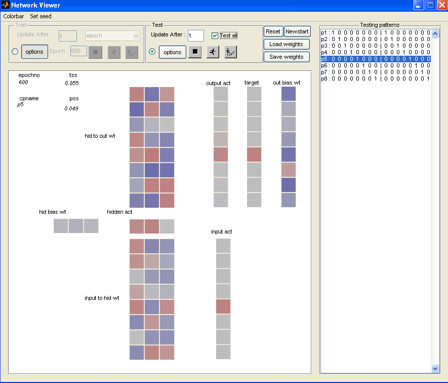
as output, through a distributed hidden representation. Over the course of this tutorial, you will create a network that learns this mapping, with the finished network illustrated in Figure B.6.
Creating a network involves four main steps, each of which is explained in a section:
While this tutorial does a complete walkthrough of setting up an auto-encoder in PDPtool, in the interest of brevity, many of the commands and options of PDPtool are left unmentioned. You are encouraged to use the PDPtool User’s Guide (Appendix C) as a more complete reference manual.
The first thing you need to do is create your own network specification. A network specification is a file with a ‘.net’ extention that specifies the architecture of your network. Such a file can be created by typing matlab commands, and can be edited using the Matlab editor. However, the easiest way to create such a file is to use the GUI.
It may be best to create a new directory for your example. So, at the command line interface type
Then change to this directory
and launch the pdp tool, by typing
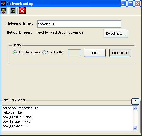
In the main pdp window, select “Create...” from the Network pull-down menu. In the “Network Name” box, enter “encoder838” (or whatever you want to name your network). The “Network Type” is Feed-forward Back propagation.
It might be useful to see the program create the “.net” file as we go along. Click the “View Script” button in the top-left corner of the window. Your “Network setup” box should look something like the one in Figure B.1. Note that one pool of units – pool(1), the bias pool, is already created for you. This pool contains a single unit that always has an activation of 1; connections from this pool to other pools implement bias weights in the network.
It is now time to define the pools you want in your network. It is good practice to do this before defining the projections. Click the “Pools” button. We must define each of the 3 pools we want (input, hidden, and output) individually. Under “Select pool type” choose “input”, then enter the name as “input” with 8 units, clicking “Add” when you are finished. You must do this for the hidden and output pool as well, using 3 and 8 units respectively. At any point during this process, to see the pools previously defined, follow the directions in this footnote.1
The network will now have four pools: bias (pool 1), input (pool 2), hidden (pool 3), and output (pool 4).
Projections are defined in a similar manner. For your back propagation network, you should define the standard feedforward projections from input to hidden to output, as well as projections from the bias units. Let’s start with the bias projections. A projection is defined by selecting a pool from the sender list, one from the receiver list and then specifying how the weights will be initialized from the drop-down menu. Start by having the “Sender” be the bias and the “Receiver” be the hidden units. For a back propagation network, you should select your initial weights to be “Random” from the pull-down menu.2 However, here are what all the options do:
Once you set the options for the bias to hidden unit projections, click “OK.” In the network script, this should add some code that looks like this:
In total, your network needs 4 projections, all defined with “Random” initial weights.3
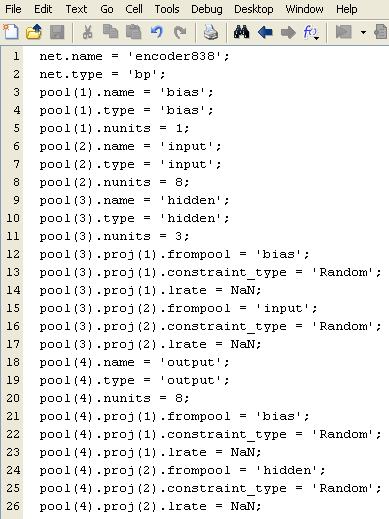
Once the projections are defined, you are done defining your network, and you are ready to continue with the other steps. Click the save button at the top of the window (the floppy disk icon), and save the file as ‘encoder838.net’. Our encoder838.net file is in Figure B.2 so you can check if yours is the same.
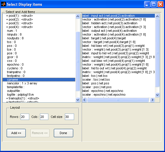
You are now ready to create the display template, which is the visualization of your network while it’s running. In the pdp window, select “Select display items...” from the “Display” drop-down menu. The window is broken into the panels: the left panel is a tree-like structure of network objects that you can add to the the display template and the right panel is your current selection of such objections.
Start by clicking “+ net: struct” since the “+” indicates it can be expanded. This shows many of the network parts. You can add networks parts that you want displayed on the template. For each item you want displayed, you need to separately add a “Label” and “Value” to the Selected Items panel. The Value will be a vector, matrix, or scalar that displays the variable of interest. The Label is a floating text box that allows you to indicate which item is which on the display.
What items do you want in your template? For any network, you want the activations of the pools displayed (except for the bias pool). This allows you to see the pattern presented and the network’s response. For many networks, if the pools are small enough (say less than 10 units each), you may want to display the weights to see how the network has solved the problem. Otherwise, you can ignore adding the weights, and you can always use the Matlab command window to view the weights if wanted during learning.
For our auto-encoder, we will want to display the pool activations, the target vector, the weights, and some summary statistics. Each of these items is also going to need a label. We’ll walk you through adding the first item, and then the rest are listed so you can add them yourself. Let’s start by adding the activation of the input layer, which is pool(2). Expand the pool(2) item on the left panel, and highlight the activation field. The click the “Add” button. You must now select whether you want to add a Label or Value. We will want to add both for each object. Thus, since Label is already selected, type the desired label, which should be short (we use “input act”). Click “Ok”. The label you added should appear in the right panel. All we did was add a text object that says “input act,” now we want to add the actual activation vector to the display. Thus, click add again on the pool(2).activation field, select Value, and set the Orientation to Vertical. The orientation determines whether the vector is a row or column vector on the template. This orientation can be important to making an intuitive display, and you may want to change it for each activation vector. Finally, set the vcslope parameter to be .5. Vcslope is used to map values (such as activations or weights) to the color map, controlling the sensitivity of the color around zero. We use .5 for activations and .1 for weights in this network. Details of this parameter are in the PDPtool User’s Guide (Appendix C).
For the auto-encoder network, follow the orientations we have selected. If you make a mistake when adding an item Value or Label, you can highlight it in the right panel and press “Remove”.
Now it’s time to add the rest of the items in the network. For each item, follow all the steps above. Thus, for each item, you need to add a Label and then the Value with the specified orientation. We list each item below, where the first one is the input activation that we just took care of. Your screen should look like Figure B.3 when you are done adding the items (however, this screen does not indicate whether or not you have the orientations or transposes the same way that I do, but this will make a difference in a second).
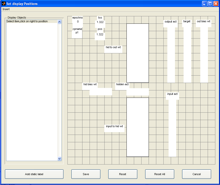
After adding these items, click “Done” if your screen looks like Figure B.3. The “Set display Positions” screen should then pop-up, where you get to place the items on the template. An intuitive way to visualize this encoder network is shown in Figure B.4. To place an item on the template, select it on the left panel. Then, right click on the grid to place the item about there, and you can then drag to the desired position. If you want to return the item to the left panel, click “Reset” with the item highlighted.
An example file is the file that defines the stimuli for the network. In the case of a feed-forward back propagation network like the one we are creating, this consists of defining a set of input-teacher pattern pairs. The file should be a series of lines formated as follows: “name input teacher”, where the name is the name of each pattern. The set of 8 unary input patterns, and their teachers (which is the same as the input pattern) are shown below. All you need to do is simply copy this segment of text into a text file, and save it as “unary.pat”. To create a new text file within Matlab, click the “New M-File” button at the top left corner of the Matlab window.
Now, all of the heavy lifting is done! It is possible to run your network using the main pdp window, loading the script, the patterns, the template, and setting the train options. However, it is much easier if you have a script that does all of this for you. Then, your network can be setup with all the right parameters with a single command.
There are two ways to do this. (1) By setting up and launching your network in the main pdp window, PDPTool will log the underlying commands in a .m file that you can run later to repeat the steps. (2) You can simply type the appropriate setup commands by hand in a .m file.
Here, we’ll describe describe the first method and provide the generated .m file (Figure B.5). Thus, you can also opt to simply type the content of Figure B.5 by hand if you prefer the second method.
Close the pdp program entirely. When you open the pdp program, your next series of actions will be recorded in the log file. First, type
which starts the pdp program. First, click “Load script”, and select the encoder838.net file that contains your network setup (Section B.1). Second, click “Load pattern” to load the unary.pat file you created (Section B.3) as both the testing and training patterns. Third, click the Display menu and select “Load Template,” selecting the encoder838.tem you created in Section B.2.
Also, you will want to select Training options that are reasonable for this network, which will become the parameters used when the network starts up with this script. Select the “Network” menu then “Training options.” The defaults are fine for this network, but they may have to be changed when setting up a custom network. For advice on setting some crucial parameters, such as the lrate and wrange, see the hints for setting up your own network in the back propagation chapter (Ex 5.4 Hints). When done adjusting training options, click “Apply” and then “OK.”
We are ready to launch the network, which is done by selecting “Launch network window” from the “Network” menu. The Network Viewer should pop up, resembling Figure B.6 (except that the network in this figure has already been trained).
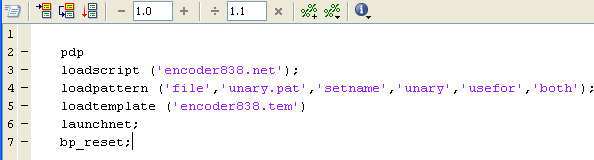
Finally, click “Reset,” which is necessary for certain parameters such as “wrange” to take effect. Now, all the actions you have just completed should be logged, in order, in a .m file in your current directory. The file will be called “pdplog#.m”, where the # will be the largest number in the directory (indicating the most recent log file created). Your file should look like Figure B.5. If your file does not look exactly like the figure, you can modify it to be exact (it’s possible you have an extra command inserted on top of the file, for instance).
You should rename the file to be “bpencoder.m”. Then you can initialize your network at any time by simply typing
in the Matlab command window, and the Network Viewer should pop-up.
That’s it; the network is finished. Train the network and see how it uses the hidden layer to represent the eight possible input patterns.