Running the test

This test case is run with the command

make test

The simulation runs for 500 time steps (suntans.dat: nsteps = 500) with a time step size of 0.2 s (suntans.dat: dt = 0.2). For this grid, given that the Voronoi distance for the equilateral triangles with sides of length $\Delta x=L/200$ is $D_g = \Delta x/\sqrt{3} = 0.2887$ m, and the maximum velocity is roughly $u_{max}=0.5$ m s$^{-1}$ (it actually never exceeds $0.44$ m s$^{-1}$), the horizontal Courant number is $C_x=u_{max}\Delta t/D_g = 0.35$, and the vertical Courant number is $C_z=w_{max}\Delta t/\Delta z_{min}=0.2\mbox{m s}^{-1} 0.2\mbox{s}/0.78 m=0.05$. Because central differencing is employed for advection of momentum (suntans.dat: nonlinear = 2), the horizontal grid Peclet number must satisfy the one-dimensional stability criterion which requires that $Pe_{\Delta x}<2/C_x$. This is an approximation and is not as restrictive as it should be for multidimensional, unstructured-grid problems, but it serves as a good approximation (See Fletcher [1] for details). For the horizontal stability, then, this requires that $\nu_H\ge u_{max}^2\Delta t/2 = 0.025$ m$^2$ s$^{-1}$ (suntans.dat: nuH = 0.025). Likewise, for vertical stability, $\nu = 0.016$ m$^2$ s$^{-1}$ (suntans.dat: nu = 0.016).

The results can be viewed with the sunplot gui from the main source directory with

./sunplot --datadir=examples/lockexchange/data

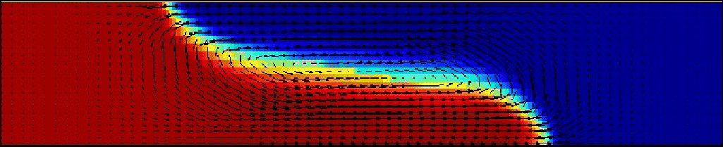
This will open up a planview of the one-dimensional grid of equilateral triangles, showing that there are 26 (1+nsteps/ntout) time steps to plot. To view the profile plot, depress the button with the middle mouse button. The last time step of the velocity vectors along with the salinity field can be viewed with the following buttons:

1. Right mouse on : To get to last time step.
2. Left mouse on : Turn on velocity vectors.
3. 3$\times$ Right mouse on : Increase vector length by a factor of 8.
4. 2$\times$ Left mouse on : Increase iskip to 3 to plot every third vector for clarity.

The display should appear as it does in Figure 10.

Figure 10: Sunplot display of the lock exchange example after 500 time steps.

0.6