NMF Algorithm
Optimization:
For  ,
,
 and
and  ,
let
,
let  ,
,
 be the
squared
be the
squared  Distances of
  from the convex envelope
of the rows of
from the convex envelope
of the rows of  and the set
  , respectively. Namely, letting
  be the standard
  –simplex, we let

Using this notation, if  is the matrix with data points
  and
and  is the matrix with archetypes
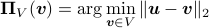
 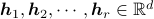 as their rows, we attempt to solve the following nonconvex problem:
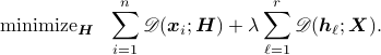
We propose an initialization algorithm based on the Successive projections algorithm in a paper by Araùjo et al. In addition, Proximal Alternating Linearized Minimization (PALM) proposed in this work by Bolte et al. is used for minimizing the above cost function.
Input: Data  ,
,  , integer
  ;
;
Output: Initial archetypes  ;
;
Set
 ;
;Set
 ;
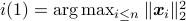
; For
Define
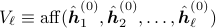 , the affine hull of
 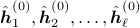 ;
;Set
 ;
;Set
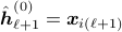 ;
;
Return
.
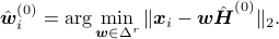
After finding the initial set of archetypes
,
initial set of weights  can be found by
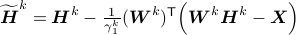
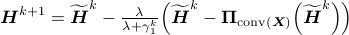
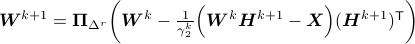
After finding the above initial estimates, we perform the PALM
iterations that is guaranteed to converge to
critical points of the risk function. For ,
and , If we let
denote the projection of on ,
for this risk
function the iterations will take the
following form:
Let  represent the
convex envelope of the rows of
represent the
convex envelope of the rows of  and
Initialize
and
Initialize  . While
 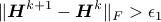 ,
, 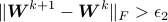 :
:
 ;
; ;
; ;
; .
.
In our code, we have also provided
an accelerated version of the
PALM iterations by employing
the technique used by Beck and Teboulle in
MFISTA in this paper
and the extension of this technique presented
by Li and Lin in this paper.
Our code gives this option to the user to choose the parameter
 or let the algorithm to decide an appropriate
value for using a data driven procedure explained below.
or let the algorithm to decide an appropriate
value for using a data driven procedure explained below.
How we choose parameter :
Let  be the singular value decomposition of the data matrix with
 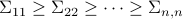 .
Taking
.
Taking  such that
  for
for  and
and
 for
for  , we let
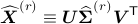
be the rank- PCA
approximation for and
be its corresponding error.
Starting from  we increase the value of in a grid of values until we reach
  as
the smallest such that
as
the smallest such that

for some constant  . The user can choose this
constant. The default is set to
. The user can choose this
constant. The default is set to  in the code.