Lecture 6: Big O and Asymptotic Analysis
CS 106B: Programming Abstractions
Spring 2023, Stanford University Computer Science Department
Lecturer: Chris Gregg, Head CA: Neel Kishnani
Slide 2
Announcements
- Assignment 2 was released on Friday.
- Now that you have submitted Assignment 1, your section leaders will be grading them throughout the week and will schedule an Interactive Grading session with you to go over your grade. IG attendance is part of your section participation grade, so please make sure to attend!
- The add/drop deadline is coming up on Friday at 5pm PDT - if you want to chat about what the class is going to look like going forward, feel free to reach out to the course staff and we'd be happy to discuss it.
-
Please see the announcement below about SOLE LaIR:

Slide 3
Computational Complexity
- How does one go about analyzing programs to compare how the program behaves as it scales? E.g., let's look at a
vectorMax()function:int vectorMax(Vector<int> &v){ int currentMax = v[0]; int n = v.size(); for (int i = 1; i < n; i++){ if (currentMax < v[i]) { currentMax = v[i]; } } return currentMax; } - What is
n? Why is it important to this function? - If we want to see how this algorithm behaves as
nchanges, we could do the following:- Code the algorithm in C++
- Determine, for each instruction of the compiled program the time needed to execute that instruction (need assembly language)
- Determine the number of times each instruction is executed when the program is run.
- Sum up all the times we calculated to get a running time.
- Steps 1-4 might work, but it is complicated, especially for today’s machines that optimize everything “under the hood.” (and reading assembly code takes a certain patience).
Slide 4
Assembly Code for the vectorMax function
0x000000010014adf0 <+0>: push %rbp
0x000000010014adf1 <+1>: mov %rsp,%rbp
0x000000010014adf4 <+4>: sub $0x20,%rsp
0x000000010014adf8 <+8>: xor %esi,%esi
0x000000010014adfa <+10>: mov %rdi,-0x8(%rbp)
0x000000010014adfe <+14>: mov -0x8(%rbp),%rdi
0x000000010014ae02 <+18>: callq 0x10014aea0 <std::__1::basic_ostream<char, std::__1::char_traits<char> >::operator<<(long)+32>
0x000000010014ae07 <+23>: mov (%rax),%esi
0x000000010014ae09 <+25>: mov %esi,-0xc(%rbp)
0x000000010014ae0c <+28>: mov -0x8(%rbp),%rdi
0x000000010014ae10 <+32>: callq 0x10014afb0 <std::__1::basic_ostream<char, std::__1::char_traits<char> >::operator<<(long)+304>
0x000000010014ae15 <+37>: mov %eax,-0x10(%rbp)
0x000000010014ae18 <+40>: movl $0x1,-0x14(%rbp)
0x000000010014ae1f <+47>: mov -0x14(%rbp),%eax
0x000000010014ae22 <+50>: cmp -0x10(%rbp),%eax
0x000000010014ae25 <+53>: jge 0x10014ae6c <vectorMax(Vector<int>&)+124>
0x000000010014ae2b <+59>: mov -0xc(%rbp),%eax
0x000000010014ae2e <+62>: mov -0x8(%rbp),%rdi
0x000000010014ae32 <+66>: mov -0x14(%rbp),%esi
0x000000010014ae35 <+69>: mov %eax,-0x18(%rbp)
0x000000010014ae38 <+72>: callq 0x10014aea0 <std::__1::basic_ostream<char, std::__1::char_traits<char> >::operator<<(long)+32>
0x000000010014ae3d <+77>: mov -0x18(%rbp),%esi
0x000000010014ae40 <+80>: cmp (%rax),%esi
0x000000010014ae42 <+82>: jge 0x10014ae59 <vectorMax(Vector<int>&)+105>
0x000000010014ae48 <+88>: mov -0x8(%rbp),%rdi
0x000000010014ae4c <+92>: mov -0x14(%rbp),%esi
0x000000010014ae4f <+95>: callq 0x10014aea0 <std::__1::basic_ostream<char, std::__1::char_traits<char> >::operator<<(long)+32>
0x000000010014ae54 <+100>: mov (%rax),%esi
0x000000010014ae56 <+102>: mov %esi,-0xc(%rbp)
0x000000010014ae59 <+105>: jmpq 0x10014ae5e <vectorMax(Vector<int>&)+110>
0x000000010014ae5e <+110>: mov -0x14(%rbp),%eax
0x000000010014ae61 <+113>: add $0x1,%eax
0x000000010014ae64 <+116>: mov %eax,-0x14(%rbp)
0x000000010014ae67 <+119>: jmpq 0x10014ae1f <vectorMax(Vector<int>&)+47>
0x000000010014ae6c <+124>: mov -0xc(%rbp),%eax
0x000000010014ae6f <+127>: add $0x20,%rsp
0x000000010014ae73 <+131>: pop %rbp
0x000000010014ae74 <+132>: retq
Slide 5
Algorithm Analysis: Primitive Operations
- Instead of those complex steps, we can define primitive operations for our C++ code.
- Assigning a value to a variable
- Calling a function
- Arithmetic (e.g., adding two numbers)
- Comparing two numbers
- Indexing into a Vector
- Returning from a function
- We assign "1 operation" to each step. We are trying to gather data so we can compare this to other algorithms.
Slide 6
Algorithm Analysis: Primitive Operations
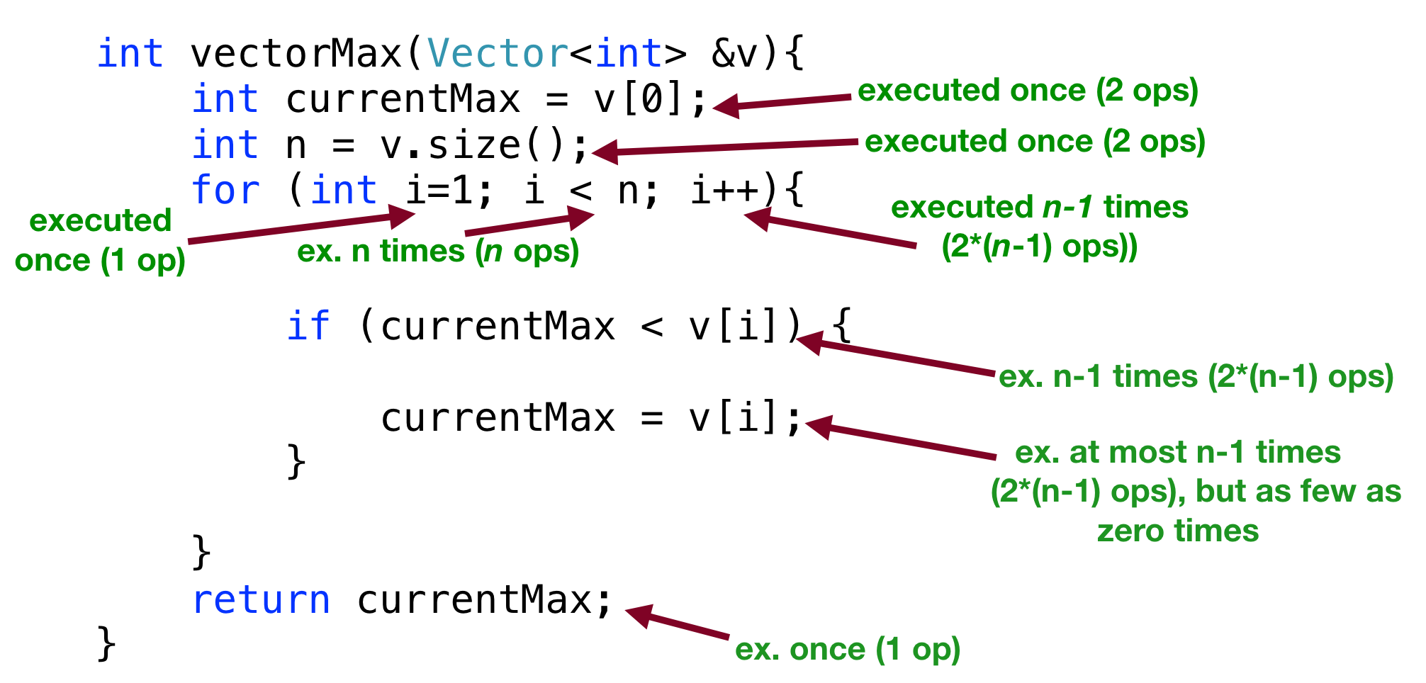
- Specifically, we can count up the primitive operations:
currentMax = v[0]has two operations (variable assignment and indexing into a Vector) and is executed once (total operations so far = 2)n = v.size()has two operations (variable assignment and calling a function) and is executed once (total operations so far: 4)- The
int i = 1in theforloop declaration is executed once, with 1 operation (total = 5) - The
i < nin thefordeclaration is executedntimes (total: n + 5) - The
i++in thefordeclaration is executedn - 1times, and is two operations (arithmetic and assignment) (total: 3n + 3 operations so far) if (currentMax < v[i])is executedn - 1times and is two operations (comparison and vector indexing) (total: 5n + 1)currentMax = v[i]is executed at mostn - 1times, and is two operations (assignment and vector indexing) but as few as zero times (if we never have to update the max!) (total: either 7n - 1 operations or 5n + 1 operations)return currentMaxis executed once, and is one operation (returning from a function) (total operations: either 7n or 5n + 2)
Slide 7
Algorithm Analysis: Primitive Operations
- Summary:
- Primitive operations for vectorMax():
- at least:
2 + 2 + 1 + n + 2 * (n - 1) + 2 * (n - 1) + 1 = 5n + 2 - at most:
2 + 2 + 1 + n + 2 * (n - 1) + 2 * (n - 1) + 2 * (n - 1) + 1 = 7n
- at least:
- i.e., if there are
nitems in the Vector, there are between5n + 2operations and7noperations completed in the function.
- Primitive operations for vectorMax():
- In other words: the best case number of operations is
5n + 2and the worst case number of operations is 7n.
Slide 8
Algorithm Analysis: Simplify!
- Do we really need this much detail? Nope!
- Let's simplify: we want a big picture approach.
- It is enough to know that
vectorMax()grows
linearly proportional ton - In other words, as the number of elements increases, the algorithm has to do proportionally more work, and that relationship is linear. 8x more elements? 8x more work.
- The reason we can make this generalization is that we want to discuss the behavior for increasingly large values of
n. The details of the+ 2and even the5or7becomes irrelevant as the numbers get increasingly large.
Slide 9
Algorithm Analysis: Big O
- Our simplification uses a mathematical construct known as Big-O notation — think "O" as in “on the Order of.”
- Wikipedia:
Big-O notation describes the limiting behavior of a function when the argument tends towards a particular value or infinity, usually in terms of simpler functions.
- In mathematical terms:
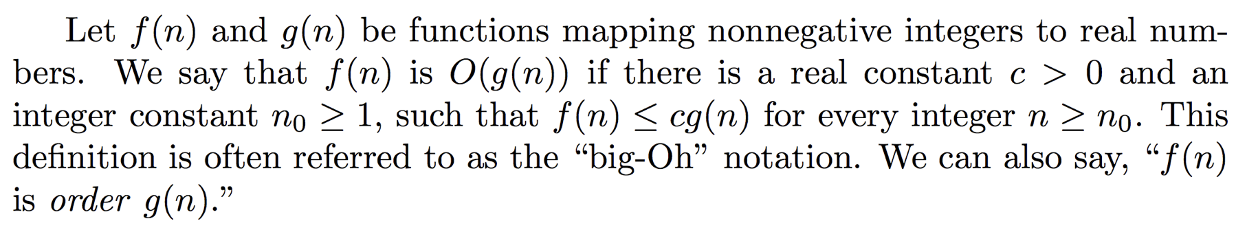
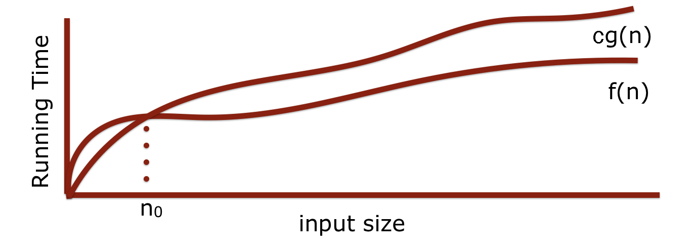
Slide 10
Algorithm Analysis: Removing constants and less significant factors
- All of the analysis on the previous few slides was actually even more than you need to worry about.
- The dirty little trick for figuring out Big-O: look at the number of steps you calculated, throw out all the constants, find the biggest factor and that’s your answer:
5n + 2 is O(n)
- Why? Because constants are not important when compared against other functions that we will cover shortly.
- In other words: for very large values of
n, there is an insignificant difference between5n + 2and, simply,n. Ifnis 1 billion, the difference between 1 billion and 5 billion and 2 is irrelevant when compared to other functions that we will see soon.
Slide 11
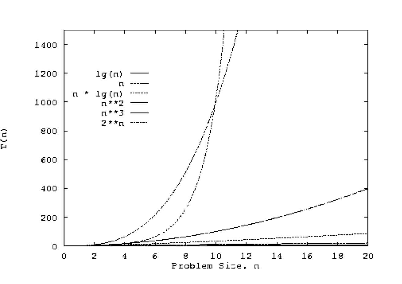
Big O: important functions
- We will care about teh following functions that appear often in data structures and algorithms:
| constant | logarithmic | linear | n log n | quadratic | polynomial (other than n2, (n^2)) |
exponential |
| O(1) | O(log n) | O(n) | O(n log n) | O(n2), O(n^2) | O(nk), O(n^k) (where k >= 1) |
O(an), O(a^n) |
- When you are deciding what Big-O is for an algorithm or function, simplify until you reach one of these functions, and you will have your answer.
- Factors farther to the right are more important. If two or more factors from the table are in your calculation, leave only the one farthest to the right.
- Practice: what is Big-O for this function?
20n3 + 10n log n + 5
(alternate:20n^3 + 10n log n + 5) - Answer:
O(n3)
(alternate:O(n^3)) - First, strip the constants: n3 + n log n (n^3 + n log n)
-
Then, find the biggest factor: n3 (n^3)
- Practice: what is Big-O for this function?
2000 log n + 7n log n + 5 - Answer:
O(n log n) - First, strip the constants: log n + n log n
- Then, find the biggest factor: n log n
Slide 12
Algorithm Analysis: Back to vectorMax()
int vectorMax(Vector<int> &v){
  int currentMax = v[0];
  int n = v.size();
  for (int i = 1; i < n; i++){
      if (currentMax < v[i]) {
          currentMax = v[i];
      }
  }
  return currentMax;
}
- When you are analyzing an algorithm or code for its computational complexity using Big-O notation, you can ignore the primitive operations that would contribute less-important factors to the run-time. Also, you always take the worst case behavior for Big-O.
- So, for
vectorMax(): ignore the original two variable initializations, the return statement, the comparison, and the setting ofcurrentMaxin the loop. - Notice that the important part of the function is the fact that the loop conditions will change with the size of the array: for each extra element, there will be one more iteration. This is a linear relationship, and therefore
O(n).
Slide 13
Algorithm Analysis: Back to vectorMax()
int vectorMax(Vector<int> &v){
    int currentMax = v[0];
    int n = v.size();
    for (int i = 1; i < n; i++){
        if (currentMax < v[i]) {
            currentMax = v[i];
        }
    }
    return currentMax;
}
- For vectorMax(): ignore the original two variable initializations, the return statement, the comparison, and the setting of currentMax in the loop.
- Notice that the important part of the function is the fact that the loop conditions will change with the size of the array: for each extra element, there will be one more iteration. This is a linear relationship, and therefore
O(n).
Slide 14
Graphing the Data for vectorMax
- In the code for today's lecture, you can find a program that times
vectorMaxfor vector sizes between 40000 and 20,480,000 elements. Additionally, it times for the case where the first element is the maximum, and also when the last element is the maximum (and all prior elements are maximum at each iteration). The graph for those results is shown below:
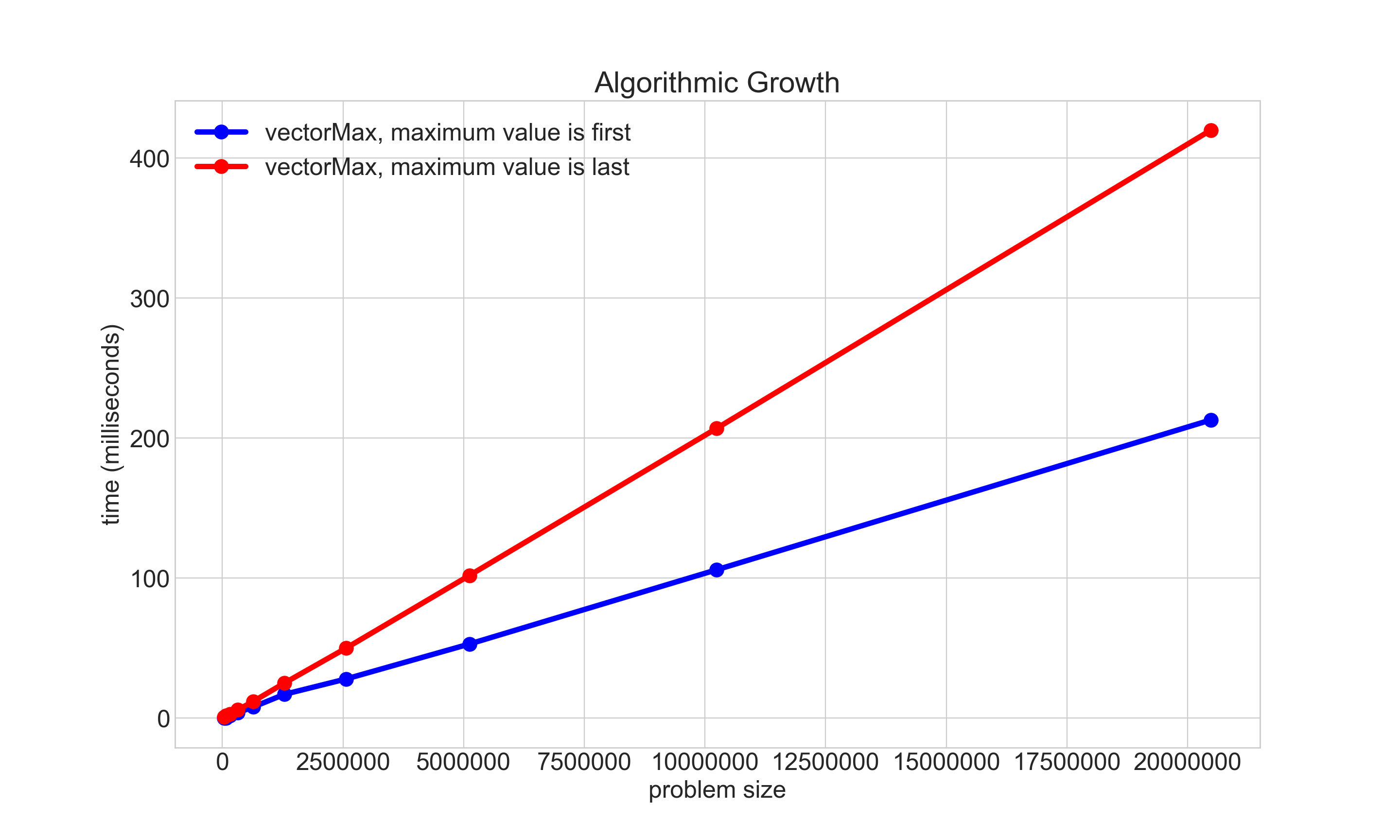
- Notice that both plots show a linear relationship!
Slide 15
Nested Loops
- Take a look at the following function, which has a nested loop:
int nestedLoop1(int n){ int result = 0; for (int i = 0; i < n; i++){ for (int j = 0; j < n; j++){ result++; } } return result; } - The inner loop (variable
j) has a complexity ofO(n), as our analysis from the previous slides would show. However, the entire inner loop happensntimes, as well! This squares the number of timesresultis incremented. - Now we have a quadratic relationship between
nand the time to complete the function, and this is O(n2) (alt: O(n^2)) behavior! - With O(n^2) behavior, if the size of the problem is 10 times bigger, the running time will be 100 times longer. We don't like O(n^2) behavior!
- As an example: let's say an O(n^2) function takes 5 seconds for a container with 100 elements.
- How much time would it take if we had 1000 elements?
- Answer: 500 seconds! This is because 10x more elements is (10^2)x more time!
- If we had 10000 elements, that is 100x more elements, meaning it would take (100^2)x more time, or 10,000 times as long as the original (50,000 seconds, or almost 14 hours), for only 100 times more elements. Quadratic behavior does not scale well!
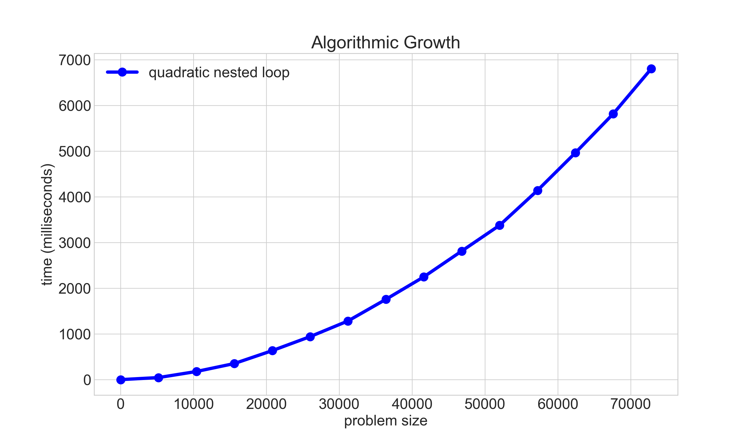
Slide 16
Plotting O(n^2) behavior
Slide 17
Cubic O(n^3) Behavior
int nestedLoop2(int n){
    int result = 0;
    for (int i = 0; i < n; i++){
        for (int j = 0; j < n; j++){
            for (int k = 0; k < n; k++) {
                result++;
            }
        }
    }
    return result;
}
- What would the complexity be of a 3-nested loop?
- Answer: O(n^3) (cubic – anything above quadratic is generally called polynomial)
- In real life, this comes up in 3D imaging, video, etc., and it is slow!
- Graphics cards are built with hundreds or thousands of processors to tackle this problem
- If it took 10 seconds for
n = 5, switching ton = 50would incur a (10^3) time increase, or 10,000 seconds!
Slide 18
Plotting O(n^2) -vs- O(n^3) behavior
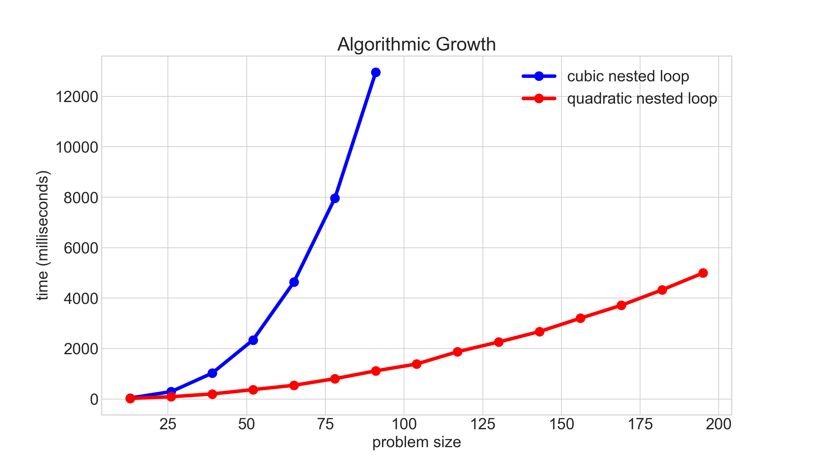
- This graph actually has an additional constant slow-down for the cubic data, simply so it could be graphed on a single chart.
Slide 19
Hidden loops
- You have to be particularly cognizant of when a data structure might be performing a looping operation without you writing the loop.
- The
Vectorclass is a good example: when you insert at the beginning of a vector, what happens?
vec before insert:
| index: | 0 | 1 | 2 | 3 |
| value: | 4 | 8 | 15 | 16 |
vec.insert(0, 100);
| index: | 0 | 1 | 2 | 3 | 4 |
| value: | 100 | 4 | 8 | 15 | 16 |
- All elements had to be moved down – how do you think this was done? With a loop inside the
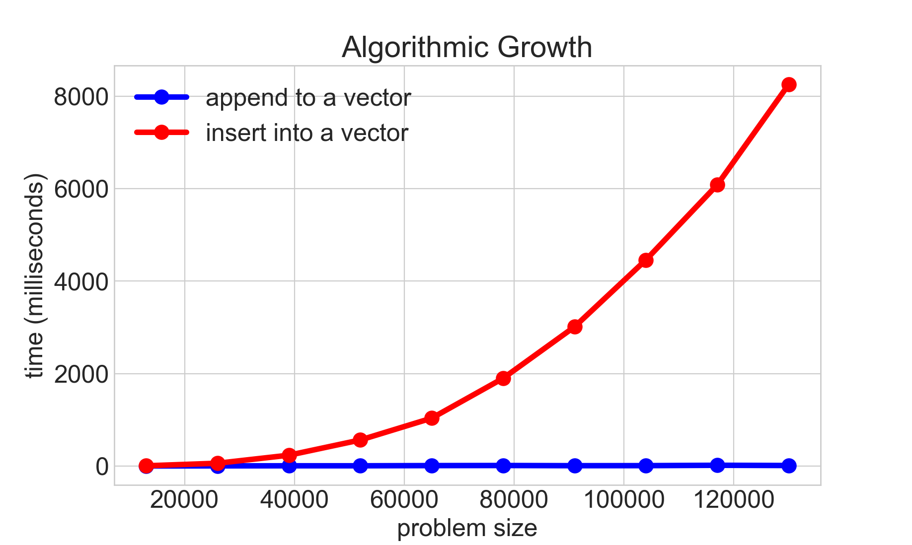
Vectorclass! - What would the complexity (big O) be of the following function?
void populateVec(Vector<int>& vec, int n) { for (int i = 0; i < n; i++) { vec.insert(0, i); } } - Answer: O(n^2), because under the hood, for each insert, the vector has to move all of the elements.
- Here is a graph of
populateVecas above, and also by replacingvec.insert(i, 0)withvec.add(i):
Slide 20
Constant Time
- When an algorithm's time is independent of the number of elements in the container it holds, this is constant time complexity, or
O(1). We love O(1) algorithms! Examples include (for efficiently designed data structures):- Adding or removing from the end of a Vector.
- Later in the course:
- Pushing onto a stack or popping off a stack.
- Enqueuing or dequeuing from a queue.
- Inserting or searching for a value in a hash table
Slide 21
Linear Search
void linearSearchVector(Vector<int>& vec, int numToFind){
    int numCompares = 0;
    bool answer = false;
    int n = vec.size();

    for (int i = 0; i < n; i++) {
        numCompares++;
        if (vec[i]==numToFind) {
            answer = true;
            break;
        }
    }
    cout << "Found? " << (answer ? "True" : "False") << ", "
         << "Number of compares: " << numCompares << endl << endl;
}
- The code above performs a linear search on a vector, to search for a particular value. What is the complexity of the function?
- Well, it depends! Let's say the number we are looking for is the first element? Then, we could say that the complexity is O(1), because it only took a single pass through the loop to find the value. Or, what if the value is the last one in the vector? Then, it would be O(n), because we had to loop through the entire vector.
- Best case: O(1)
- Worst case: O(n)
- We often only report the worst case, because we don't know what the data is, and we want to be informed about what the worst case is.
Slide 22
Binary Search
- There is another type of search that we can perform on a list that is in order: binary search (as you might have seen in 106A)
- If you have ever played a guess my number game before, you will have implemented a binary search, if you played the game efficiently!
- The game is played as follows:
- one player thinks of a number between 0 and 100 (or any other maximum).
- the second player guesses a number between 1 and 100
- the first player says "higher" or "lower," and the second player keeps guessing until they guess correctly.
- The most efficient guessing algorithm for the number guessing game is simply to choose a number that is between the high and low that you are currently bound to. Example:
bounds: 0, 100 guess: 50 (no, the answer is lower) new bounds: 0, 49 guess: 25 (no, the answer is higher) new bounds: 26, 49 guess: 38 etc. - With each guess, the search space is divided into two.
- This means that we can very quickly converge on a solution. In fact, we can converge on a solution in logarithmic time, or O(log n).
- If we played the guessing game with numbers between 1 and 128, how many guesses, maximum, would we need?
- First, we have 128 to choose from, then 64, then 32, then 16, then 8, then 4, then 2, and finally 1 – this is 8 guesses, or
log2(128) + 1. If we doubled the range to between 1 and 256, we would only have to make a single extra guess.
- First, we have 128 to choose from, then 64, then 32, then 16, then 8, then 4, then 2, and finally 1 – this is 8 guesses, or
Slide 23
Binary Search
Here is some code that performs a binary search:
void binarySearchVector(Vector<int> &vec, int numToFind) {
    int low=0;
    int high=vec.size()-1;
    int mid;
    int numCompares = 0;
    bool found=false;
    while (low <= high) {
        numCompares++;
        mid = low + (high - low) / 2; // to avoid overflow
        if (vec[mid] > numToFind) {
            high = mid - 1;
        }
        else if (vec[mid] < numToFind) {
            low = mid + 1;
        }
        else {
            found = true;
            break;
        }
    }
    cout << "Found? " << (found ? "True" : "False") << ", " <<
    "Number of compares: " << numCompares << endl << endl;
}
- The worst-case complexity of this code is
O(log n). It is technicallyO(log2 n), but we don't have to worry about logarithmic bases when looking at complexity. - The best case is O(1) (if we guess immediately)
- The general rule for determining if something is logarithmic: if the problem is one of "divide and conquer," it is logarithmic.
- If, at each stage, the problem size is cut in half (or a third, etc.), it is logarithmic.
- We love logarithmic time, because we can solve large problems very fast.
- Logarithmic time is not quite as fast as O(1) time, but it is almost always good enough, and still very fast.
Slide 24
Exponential Time
- If we love logarithmic and constant time algorithms, we hate exponential time algorithms,
O(a^n). - We will see examples of exponential time algorithms soon (when we get to recursion, in particular), but one good example is finding every possible subset of a set.
- For the set {1, 2, 3}, the possible combinations are {}, {1}, {2}, {3}, {1, 2}, {2, 3}, {1, 3}, {1, 2, 3}. For an
nof 3, we ended up having to enumerate eight different subsets, meaning that it is certainly worse than linear. Indeed, exponential problems grow very, very fast, and are often not possible to solve completely, even for relatively small values forn.
- For the set {1, 2, 3}, the possible combinations are {}, {1}, {2}, {3}, {1, 2}, {2, 3}, {1, 3}, {1, 2, 3}. For an
Slide 25
Ramifications of Big O Differences
- Here are some numbers
- If we have an algorithm that has 1000 elements, and the O(log n) version runs in 10 nanoseconds…
| constant | logarithmic | linear | n log n | quadratic | polynomial (other than n2, (n^2)) |
exponential |
| 1 nanoseconds | 10 nanoseconds | 1 microsecond | 10 microseconds | 1 millisecond | 1 second | 10^292 years |
Slide 26
Ramifications of Big O Differences
- If we have an algorithm that has 1000 elements, and the O(log n) version runs in 10 milliseconds…
| constant | logarithmic | linear | n log n | quadratic | polynomial (other than n2, (n^2)) |
exponential |
| 1 milliseconds | 10 milliseconds | 1 second | 10 seconds | 17 minutes | 277 hours | heat death of the universe |
Slide 27
Recap
- Asymptotic Analysis / Big-O / Computational Complexity
- We want a "big picture" assessment of our algorithms and functions
- We can ignore constants and factors that will contribute less to the result!
- We most often care about worst case behavior.
- We love O(1) and O(log n) behaviors!
- Big-O notation is useful for determining how a particular algorithm behaves, but be careful about making comparisons between algorithms – sometimes this is helpful, but it can be misleading.
- Algorithmic complexity can determine the difference between running your program over your lunch break, or waiting until the Sun becomes a Red Giant and swallows the Earth before your program finishes – that's how important it is!