Graph Shortest Path Algorithms
CS 106B: Programming Abstractions
Spring 2023, Stanford University Computer Science Department
Lecturer: Chris Gregg, Head CA: Neel Kishnani
Slide 2
Announcements
- Final exam, Friday!
Slide 3
Today's Topics
- We will be discussing shortest path graph algorithms, and focusing on Dijkstra's Algorithm
- Graph Shortest Path Algorithms
- Breadth First Search
- Dijkstra's algorithm, with a side-discussion about greedy algorithms
- A* Algorithm
Slide 4
Motivation
- As we saw in the last lecture, graphs are everywhere. One prime example is a road map.
- Google Maps can extremely quickly find a best-path route at any time of the day for you to get from one point to another by car, bike, foot, or public transportation. It can also update the path while you are on-route, and provide alternate suggestions.
- The way Google Maps does this incredible task is by the use of shortest-path graph searching algorithms, such as the ones we will see today.
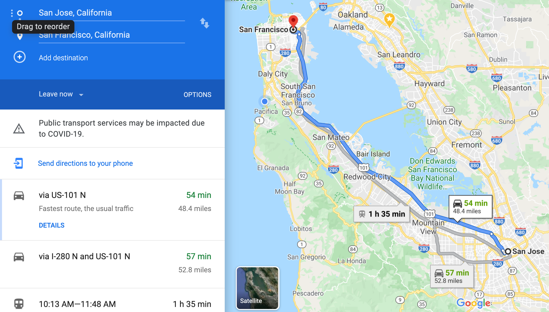
- Note on the map above that Google gives you different routes.
- You can go on the 101
- You can go on the 280
- You could go on El Camino Real if you wanted to, but Google doesn't even give you that choice because it would take so much longer
- Google priorizes by time to get to your destination, not distance, although often distance is minimized, too
- Google uses a tremendous amount of data, both historical and real-time to get you a good estimate
- Google knows all the speed limits, traffic (real-time, in many cases), stop lights, etc., and uses it all to weight their graph
Slide 5
Breadth First Search
- The first graph searching algorithm we will look at is our old friend the Breadth First Search.
- The big idea is to do the search by path-length: first, look at the neighbors of the start and see if your destination is in one of those paths.
- If not, search one more level away – the neighbors of your neighbors.
- Continue with the neighbors-of-your-neighbors-neighbors until you eventually find a path
- You will always find the shortest path in terms of number of hops, but this does not take into consideration the weights of the edges.
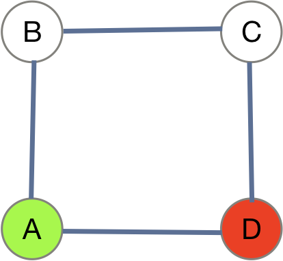
- The BFS algorithm is exactly like it has been in the past for other types of searching: you enqueue the start node into a queue, then go into a
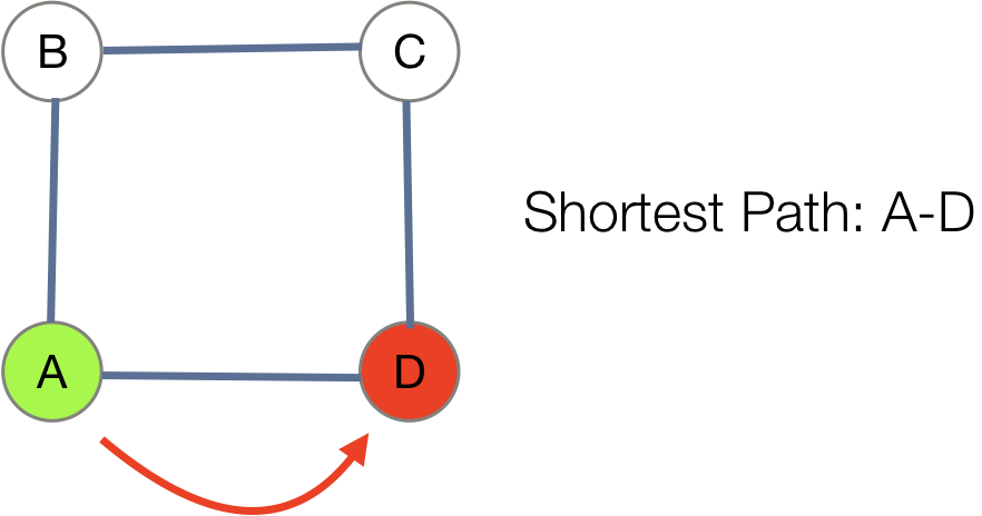
whileloop, dequeueing the first, checking for the destination, and then enqueue all neighbors. - For the graph below, a BFS from A to D simply gives us A-D as the path:
- This is the shortest path:
- Once we add weights, though, BFS no longer finds us our shortest weighted path:
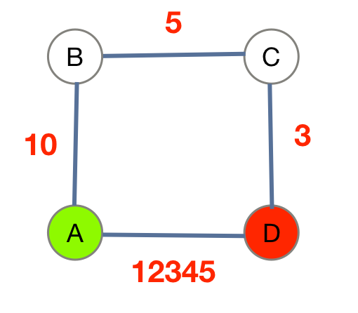
- This is the path we want:

- So: BFS works great for finding the shortest path length without considering weights, but it can break miserably with weights.
Slide 6
Greedy Algorithms
- A so-called greedy algorithm is one that prioritizes finding a solution by what is "best right now."
- In other words, a greedy algorithm looks at its options and always chooses whatever gets it closer to a solution in the best possible way given the current situation.
- Let's take a look at a simple example of a greedy algorithm: providing change for a purchase or service.
- In the U.S., we have four standard coins: the penny (1 cent), the nickel (5 cents), the dime (10 cents), and the quarter (25 cents). There are also half dollars and dollar coins, but let's stick with the four smaller coins.
- Let's make some change, say $0.47 cents. What are we going to do? Well, we start with $0.47, and then we take out a quarter. Then, we subtract $0.25 from the original, and we are left with $0.22. Then, we take a dime, and subtract that from what is left over, for a total of $0.12 cents left. Then we get another dime, and subtract $0.10 cents again, leaving us with $0.02 cents. We take out a penny, and subtract $0.01 cents, leaving us with $0.01 cents. Then we take out another penny, subtract $0.01 cents from the 1 cent remaining, and we have 0 cents. So, we give out the quarter, two dimes, and two pennies, and we have made change for $0.47 cents.
- Why did we run the algorithm in the way we did? We had choices! Why did we always start with the largest coin when we had a choice?
- We wanted to minimize the number of total coins we gave back!
- We could have always just given back pennies, but this would not have minimized the number of coins.
- This algorithm is greedy: it says, the best path right now is to take the biggest coin, and that's what it did.
Slide 7
When Greedy Algorithms Go Wrong
- Our making change example worked great as a gredy algorithm, because it always gave us the fewest coins back.
- But what if we change things around a bit? What if the U.S. added another coin, with a 12 cents denomination (call it a doz, let's say)
- What would our algorithm do if we wanted to make 45 cents change?
- First, we would choose a quarter, and we would have 1 quarter and need
45 - 25 = 20cents still. - Next, we would choose the doz, because it is the next biggest coin that is less than 20 cents. This leaves us with
20 - 12 = 8cents to make, and two coins (25 and 12) - Next, we choose a nickel, and this leaves us with
8 - 5 = 3cents to make, and three coins (25, 12, and 5) - We then have to do three more steps, choosing a penny at each step. This leaves us with six coins (25, 12, 5, 1, 1, and 1), which we give back to the customer.
- First, we would choose a quarter, and we would have 1 quarter and need
- Our algorithm did give us the correct change, but it was not optimal to give us the fewest number of coins!
- We should have chosen a quarter and two dimes, (25, 10, 10), which would have been only three coins and a better solution.
- Sometimes, greedy algorithms work, and sometimes they don't.
Slide 8
Dijkstra's Algorithm
- The second shortest-path search algorithm we are going to look at is Dijkstra's Algorithm, named after the computer scientist Edsger Dijkstra.
- Dijkstra's algorithm is greedy (and one that works), and as it progresses, it attempts to find the shortest path by choosing the best path from the available choices at each step.
- Dijkstra's algorithm can be performed in a number of ways. One method is to use a priority queue instead of a queue (as in BFS), with the priorities as the total path length so far.
- This method is virtually identical to BFS, but does require keeping track of all paths in the priority queue.
- A different form of Dijkstra's algorithm uses a table of nodes, and keeps track of how far away from the start each node is, updating by looking at neighbors of unseen nodes. It also keeps track of enough information to create the shortest path after the table is filled in.
- We will do an example with the table method.
- Example website: https://web.stanford.edu/~cgregg/graphs.html
- Example to load (click "Solution" below and then copy all text. Paste into above website after clicking
Load)
- Example to load (click "Solution" below and then copy all text. Paste into above website after clicking
{"nodes":[{"color":"green","x":195,"y":439,"name":"A"},{"color":"green","x":411,"y":439,"name":"B"},{"color":"green","x":296,"y":333,"name":"C"},{"color":"green","x":293,"y":201,"name":"D"},{"color":"green","x":178,"y":272,"name":"E"},{"color":"green","x":125,"y":124,"name":"F"},{"color":"green","x":416,"y":117,"name":"G"},{"color":"green","x":289,"y":510,"name":"SJ"},{"color":"green","x":269,"y":46,"name":"SF"}],"edges":[{"node1":{"color":"green","x":195,"y":439,"name":"A"},"node2":{"color":"green","x":289,"y":510,"name":"SJ"},"weight":5,"textX":242,"textY":461.5,"textWidth":10.0107421875,"textHeight":13,"color":"black"},{"node1":{"color":"green","x":289,"y":510,"name":"SJ"},"node2":{"color":"green","x":411,"y":439,"name":"B"},"weight":10,"textX":350,"textY":461.5,"textWidth":20.021484375,"textHeight":13,"color":"black"},{"node1":{"color":"green","x":411,"y":439,"name":"B"},"node2":{"color":"green","x":296,"y":333,"name":"C"},"weight":8,"textX":353.5,"textY":373,"textWidth":10.0107421875,"textHeight":13,"color":"black"},{"node1":{"color":"green","x":195,"y":439,"name":"A"},"node2":{"color":"green","x":296,"y":333,"name":"C"},"weight":200,"textX":245.5,"textY":373,"textWidth":30.0322265625,"textHeight":13,"color":"black"},{"node1":{"color":"green","x":296,"y":333,"name":"C"},"node2":{"color":"green","x":293,"y":201,"name":"D"},"weight":13,"textX":294.5,"textY":254,"textWidth":20.021484375,"textHeight":13,"color":"black"},{"node1":{"color":"green","x":178,"y":272,"name":"E"},"node2":{"color":"green","x":293,"y":201,"name":"D"},"weight":1,"textX":235.5,"textY":223.5,"textWidth":10.0107421875,"textHeight":13,"color":"black"},{"node1":{"color":"green","x":293,"y":201,"name":"D"},"node2":{"color":"green","x":125,"y":124,"name":"F"},"weight":5,"textX":209,"textY":149.5,"textWidth":10.0107421875,"textHeight":13,"color":"black"},{"node1":{"color":"green","x":125,"y":124,"name":"F"},"node2":{"color":"green","x":178,"y":272,"name":"E"},"weight":9,"textX":151.5,"textY":185,"textWidth":10.0107421875,"textHeight":13,"color":"black"},{"node1":{"color":"green","x":125,"y":124,"name":"F"},"node2":{"color":"green","x":269,"y":46,"name":"SF"},"weight":1,"textX":197,"textY":72,"textWidth":10.0107421875,"textHeight":13,"color":"black"},{"node1":{"color":"green","x":269,"y":46,"name":"SF"},"node2":{"color":"green","x":416,"y":117,"name":"G"},"weight":18,"textX":342.5,"textY":68.5,"textWidth":20.021484375,"textHeight":13,"color":"black"},{"node1":{"color":"green","x":293,"y":201,"name":"D"},"node2":{"color":"green","x":416,"y":117,"name":"G"},"weight":6,"textX":354.5,"textY":146,"textWidth":10.0107421875,"textHeight":13,"color":"black"},{"node1":{"color":"green","x":416,"y":117,"name":"G"},"node2":{"color":"green","x":125,"y":124,"name":"F"},"weight":2,"textX":270.5,"textY":107.5,"textWidth":10.0107421875,"textHeight":13,"color":"black"},{"node1":{"color":"green","x":416,"y":117,"name":"G"},"node2":{"color":"green","x":411,"y":439,"name":"B"},"weight":20,"textX":413.5,"textY":265,"textWidth":20.021484375,"textHeight":13,"color":"black"},{"node1":{"color":"green","x":178,"y":272,"name":"E"},"node2":{"color":"green","x":195,"y":439,"name":"A"},"weight":40,"textX":186.5,"textY":342.5,"textWidth":20.021484375,"textHeight":13,"color":"black"},{"node1":{"color":"green","x":296,"y":333,"name":"C"},"node2":{"color":"green","x":416,"y":117,"name":"G"},"weight":15,"textX":356,"textY":212,"textWidth":20.021484375,"textHeight":13}]}
- Setup:
- Create a table of all nodes, with a distance from the start as one row. A second row will be called previous, which will annotate which node we were looking at when we updated the node's distance. A final row, seen starts out with all nodes as Not Seen, and gets updated after we analyze each node in turn. Here is an example graph, representing a map where we are trying to get from San Jose to San Francisco and we have nodes A-G as potential different paths to take.
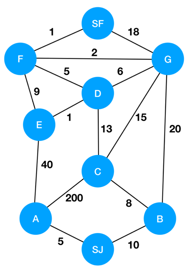
- Create a table of all nodes, with a distance from the start as one row. A second row will be called previous, which will annotate which node we were looking at when we updated the node's distance. A final row, seen starts out with all nodes as Not Seen, and gets updated after we analyze each node in turn. Here is an example graph, representing a map where we are trying to get from San Jose to San Francisco and we have nodes A-G as potential different paths to take.
- You might think, "this is going to take all day to run the algorithm!" but it is very doable.
- Here is the basic algorithm:
- Of the unseen/unvisited nodes, find the node that currently has the shortest distance from the start from the un-seen nodes.
- Look at this node's neighbors, and update the total distance to the neighbors based on their distance and the distance already to this node.
- If the node visited is the destination, stop
- Repeat from step 1.
- Here is the table we will update:
SJ A B C D E F G SF Distance from SJ 0 ∞ ∞ ∞ ∞ ∞ ∞ ∞ ∞ Previous - Seen? N N N N N N N N N - Notice:
- All the distances to SJ are listed as infinity, except for the distance from SJ to itself, which is 0. We don't yet know the distance from SJ from the other nodes, because we haven't analyzed them yet (formally – we can see them in the graph, but for our table we haven't yet analyzed anything).
- The previous row is empty
- All nodes (including SJ) are listed as Not Seen (N).
- Step 1:
- Of the unseen/unvisited nodes, find the node that currently has the shortest distance from the start from the un-seen nodes. That would be SJ (it has a distance of 0, and all others have a distance of ∞).
- Look at SJ's neighbors, A and B. Both can be reached from SJ by their respective distances, and both are less than ∞. So we update the table, and then we mark SJ as visited. We also update Previous to show that we got to A and B directly from SJ:
                 SJ   A    B    C    D    E    F    G    SF
Distance from SJ 0    5    10   ∞    ∞    ∞    ∞    ∞    ∞
Previous         -    SJ   SJ
Seen?            Y    N    N    N    N    N    N    N    N
- Step 2:
- Of the unseen/unvisited nodes, find the node that currently has the shortest distance from the start from the un-seen nodes. Now this is A.
- Look at A's neighbors, SJ, C, and E. SJ has been visited, so we ignore it. We update E to have a distance of
5 + 40from SJ (because we have already gone 5 to get to A). We update C to be 205.
                 SJ   A    B    C    D    E    F    G    SF
Distance from SJ 0    5    10   205  ∞    45   ∞    ∞    ∞
Previous         -    SJ   SJ   A         A
Seen?            Y    Y    N    N    N    N    N    N    N
- Step 3:
- Of the unseen/unvisited nodes, find the node that currently has the shortest distance from the start from the un-seen nodes. Now this is B.
- Look at B's neighbors, SJ, C, and G. We recognize that SJ-B-C is going to be shorter than SJ-A-C becuase
10 + 8 = 18is shorter than205. So, we update C to have a distance of18and we modify its Previous to be from B. We update G to be 30.
                 SJ   A    B    C    D    E    F    G    SF
Distance from SJ 0    5    10   18   ∞    45   ∞    30   ∞
Previous         -    SJ   SJ   B         A         B
Seen?            Y    Y    Y    N    N    N    N    N    N
- Step 4:
- Of the unseen/unvisited nodes, find the node that currently has the shortest distance from the start from the un-seen nodes. Now this is C.
- Look at C's neighbors, A, B, D, and G. We ignore A and B (already seen). We make D
18 + 13 = 31and we see that we don't need to udpate G because18 + 15 = 33is greater than30.
                 SJ   A    B    C    D    E    F    G    SF
Distance from SJ 0    5    10   18   31   45   ∞    30   ∞
Previous         -    SJ   SJ   B    C    A         B
Seen?            Y    Y    Y    Y    N    N    N    N    N
- Step 5:
- Of the unseen/unvisited nodes, find the node that currently has the shortest distance from the start from the un-seen nodes. Now this is G.
- Look at G's neighbors, B, C, D, F, and SF. We ignore B and C. We don't update D (already smaller than 36), we update F to be 32, and we update SF to be 48. We can't stop yet, even though we have reached SF! This is because we may have a shorter path.
                 SJ   A    B    C    D    E    F    G    SF
Distance from SJ 0    5    10   18   31   45   32   30   48
Previous         -    SJ   SJ   B    C    A    G    B    G
Seen?            Y    Y    Y    Y    N    N    N    Y    N
- Step 6:
- Of the unseen/unvisited nodes, find the node that currently has the shortest distance from the start from the un-seen nodes. Now this is D.
- Look at D's neighbors, C, E, F, and G. We ignore C and G. We update E to be 32, because
31 + 1 = 32and this is less than 45. We don't update F (already shorter than 36).
                 SJ   A    B    C    D    E    F    G    SF
Distance from SJ 0    5    10   18   31   32   32   30   48
Previous         -    SJ   SJ   B    C    D    G    B    G
Seen?            Y    Y    Y    Y    Y    N    N    Y    N
- Step 7:
- Of the unseen/unvisited nodes, find the node that currently has the shortest distance from the start from the un-seen nodes. Now this is either E or F, and it doesn't matter which one we choose. Let's choose E.
- Look at E's neighbors, A, D, and F. We ignore A and D. We don't update F. Notice that we have to do less updating as we get further through the graph!
                 SJ   A    B    C    D    E    F    G    SF
Distance from SJ 0    5    10   18   31   32   32   30   48
Previous         -    SJ   SJ   B    C    D    G    B    G
Seen?            Y    Y    Y    Y    Y    Y    N    Y    N
- Step 8:
- Of the unseen/unvisited nodes, find the node that currently has the shortest distance from the start from the un-seen nodes. Now this is either F.
- Look at F's neighbors, D, E, G, and SF. We ignore D, E, and G. We update SF because
32 + 1 = 33is less than48. So, we did need to update SF after all!
                 SJ   A    B    C    D    E    F    G    SF
Distance from SJ 0    5    10   18   31   32   32   30   33
Previous         -    SJ   SJ   B    C    D    G    B    F
Seen?            Y    Y    Y    Y    Y    Y    Y    Y    N
- Step 9:
- Find the shortest distance from the start from the un-seen nodes: now this is SF (it might not always be the last node, but happens to be so in this case).
- Because we are visiting the destination, we know that we have found the shortest path. We are done, and the shortest path is 33.
                 SJ   A    B    C    D    E    F    G    SF
Distance from SJ 0    5    10   18   31   32   32   30   33
Previous         -    SJ   SJ   B    C    D    G    B    F
Seen?            Y    Y    Y    Y    Y    Y    Y    Y    Y
- Now, to get the actual path, we simply follow the Previous nodes backwards from SF:
- SF's previous was F
- F's previous was G
- G's previous was B
- B's previous was SJ
- Therefore, the shortest path is
SJ -> B -> G -> F -> SFwith a length of 33.
Slide 9
A* Search
- One of the downsides to Dijkstra's algorithm is that it can, in many circumstances, ignore other sources of information that might prove useful to finding the shortest path in the fewest number of steps.
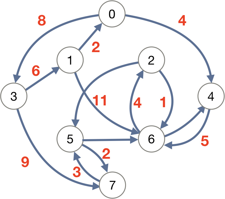
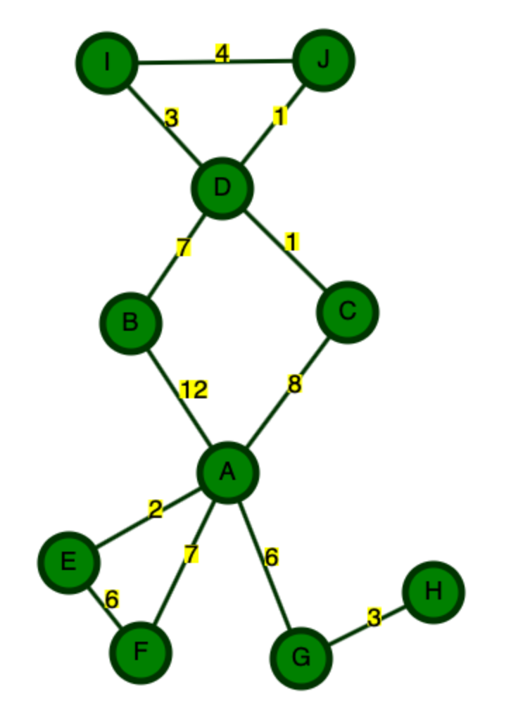
- For example, take a look at the following graph, where we want to find the shortest path from
AtoJ. If all we have is the graph in this form, Dijkstra's is the best we can do. - But, what if we know that this is a map, and that any paths to the south of A are probably going to take us in the wrong direction? Yes, it could be the case that those would lead to a shorter path, but on a real map, it is unlikely that going to far South when your destination is to the North is going to lead to the shortest path.
- We call the idea of using external information about a graph a heuristic. The heuristic estimates the cost of the cheapest path to the goal. It is different for every problem.
- A heuristic should always underestimate the distance to the goal. If it overestimates the distance, it could end up finding a solution that is not actually optimal (though it will do so relatively fast).
- We use the heuristic as an addition to the value for the priority.
- For the case of maps, if the distance to the destination is closer, this will weight the nodes in that direction to be preferable (i.e., they will actually have a lower priority calculation).
- In other words,
priority(u) = weight(s, u) + heuristic(u, d), wheresis the start,uis the node we are considering, anddis the destination.
Slide 10
A* Search example
- Example website: https://web.stanford.edu/~cgregg/graphs.html
- Example to load (click "Solution" below and then copy all text. Paste into above website after clicking
Load)
- Example to load (click "Solution" below and then copy all text. Paste into above website after clicking
{"nodes":[{"color":"green","x":292,"y":355,"name":"A"},{"color":"green","x":223,"y":249,"name":"B"},{"color":"green","x":377,"y":241,"name":"C"},{"color":"green","x":288,"y":153,"name":"D"},{"color":"green","x":179,"y":419,"name":"E"},{"color":"green","x":230,"y":483,"name":"F"},{"color":"green","x":344,"y":487,"name":"G"},{"color":"green","x":438,"y":440,"name":"H"},{"color":"green","x":206,"y":64,"name":"I"},{"color":"green","x":360,"y":62,"name":"J"}],"edges":[{"node1":{"color":"green","x":292,"y":355,"name":"A"},"node2":{"color":"green","x":344,"y":487,"name":"G"},"weight":6,"textX":318,"textY":408,"textWidth":10.0107421875,"textHeight":13,"color":"black"},{"node1":{"color":"green","x":344,"y":487,"name":"G"},"node2":{"color":"green","x":438,"y":440,"name":"H"},"weight":3,"textX":391,"textY":450.5,"textWidth":10.0107421875,"textHeight":13,"color":"black"},{"node1":{"color":"green","x":292,"y":355,"name":"A"},"node2":{"color":"green","x":230,"y":483,"name":"F"},"weight":7,"textX":261,"textY":406,"textWidth":10.0107421875,"textHeight":13,"color":"black"},{"node1":{"color":"green","x":230,"y":483,"name":"F"},"node2":{"color":"green","x":179,"y":419,"name":"E"},"weight":6,"textX":204.5,"textY":438,"textWidth":10.0107421875,"textHeight":13,"color":"black"},{"node1":{"color":"green","x":292,"y":355,"name":"A"},"node2":{"color":"green","x":179,"y":419,"name":"E"},"weight":2,"textX":235.5,"textY":374,"textWidth":10.0107421875,"textHeight":13,"color":"black"},{"node1":{"color":"green","x":292,"y":355,"name":"A"},"node2":{"color":"green","x":377,"y":241,"name":"C"},"weight":8,"textX":334.5,"textY":285,"textWidth":10.0107421875,"textHeight":13,"color":"black"},{"node1":{"color":"green","x":292,"y":355,"name":"A"},"node2":{"color":"green","x":223,"y":249,"name":"B"},"weight":12,"textX":257.5,"textY":289,"textWidth":20.021484375,"textHeight":13,"color":"black"},{"node1":{"color":"green","x":223,"y":249,"name":"B"},"node2":{"color":"green","x":288,"y":153,"name":"D"},"weight":7,"textX":255.5,"textY":188,"textWidth":10.0107421875,"textHeight":13,"color":"black"},{"node1":{"color":"green","x":377,"y":241,"name":"C"},"node2":{"color":"green","x":288,"y":153,"name":"D"},"weight":1,"textX":332.5,"textY":184,"textWidth":10.0107421875,"textHeight":13,"color":"black"},{"node1":{"color":"green","x":288,"y":153,"name":"D"},"node2":{"color":"green","x":360,"y":62,"name":"J"},"weight":1,"textX":324,"textY":94.5,"textWidth":20.021484375,"textHeight":13,"color":"black"},{"node1":{"color":"green","x":288,"y":153,"name":"D"},"node2":{"color":"green","x":206,"y":64,"name":"I"},"weight":3,"textX":247,"textY":95.5,"textWidth":10.0107421875,"textHeight":13,"color":"black"},{"node1":{"color":"green","x":206,"y":64,"name":"I"},"node2":{"color":"green","x":360,"y":62,"name":"J"},"weight":4,"textX":283,"textY":50,"textWidth":10.0107421875,"textHeight":13,"color":"black"}]}
- Let's look at this graph with Dijkstra, first. We want to find the shortest path from
AtoJ.
                  A    B    C    D    E    F    G    H   I   J
Distance from A   0    ∞    ∞    ∞    ∞    ∞    ∞    ∞   ∞   ∞
Previous          -
Seen?             N    N    N    N    N    N    N    N   N   N

Dijkstra:
1.(A)             A    B    C    D    E    F    G    H   I   J
Distance from A   0    12   8    ∞    2    7    6    ∞   ∞   ∞
Previous          -    A    A         A    A    A
Seen?             Y    N    N    N    N    N    N    N   N   N

2.(E)             A    B    C    D    E    F    G    H   I   J
Distance from A   0    12   8    ∞    2    7    6    ∞   ∞   ∞
Previous          -    A    A         A    A    A
Seen?             Y    N    N    N    Y    N    N    N   N   N

3.(G)             A    B    C    D    E    F    G    H   I   J
Distance from A   0    12   8    ∞    2    7    6    9   ∞   ∞
Previous          -    A    A         A    A    A    G
Seen?             Y    N    N    N    Y    N    Y    N   N   N

4.(F)             A    B    C    D    E    F    G    H   I   J
Distance from A   0    12   8    ∞    2    7    6    7   ∞   ∞
Previous          -    A    A         A    A    A    G
Seen?             Y    N    N    N    Y    Y    Y    N   N   N

5.(H)             A    B    C    D    E    F    G    H   I   J
Distance from A   0    12   8    ∞    2    5    6    7   ∞   ∞
Previous          -    A    A         A    A    A    G
Seen?             Y    N    N    N    Y    Y    Y    Y   N   N

6.(C)             A    B    C    D    E    F    G    H   I   J
Distance from A   0    12   8    ∞    2    5    4    7   ∞   ∞
Previous          -    A    A         A    A    A    G
Seen?             Y    N    N    N    Y    Y    Y    Y   N   N
...
- We'll stop calculating after 6 steps, as you can see the pattern (as in the other Dijkstra example). There would be many more steps to get all the way to J.
- Notice that the shortest paths at the beginning are all below A. If we know this is a map, why are we going South?
- We can use a heuristic based on the straight-line-distance to
Jfrom all other nodes. In this case, we're dividing the pixel distance by the shortest pixel distance for all non-J nodes.
A*
Distances to J and divided by the smallest distance (116)
A 301, 2.6
B 232, 2
C 180, 1.6
D 116, 1
E 400, 3.4
F 441, 3.8
G 425, 3.7
H 386, 3.3
I 154, 1.3
J 0, 0
Now, when we run the algorithm, we use the Distance + future distance to pull out of the priority queue. We still update the real lengths when we update the actual Distance from A, so that we have the real distances. The heuristic is just helping us with the calculation.
A*:
                    A      B      C      D      E      F     G     H     I     J
Distance from A     0      ∞      ∞      ∞      ∞      ∞     ∞     ∞     ∞     ∞
Distance + future   2.6
Previous            -
Seen?               N      N      N      N      N      N     N     N     N     N

1(A)                A      B      C      D      E      F     G     H     I     J
Distance from A     0      12      8     ∞      2      7     6     ∞     ∞     ∞
Distance + future   2.6    14     9.6           5.4    11.8  9.7
Previous            -
Seen?               Y      N      N      N      N      N     N     N     N     N

2(E)                A      B      C      D      E      F     G     H     I     J
Distance from A     0      12     8      ∞      2      7     6     ∞     ∞     ∞
Distance + future   2.6    14     9.6           5.4    11.8  9.7
Previous            -      A      A             A      A     A
Seen?               Y      N      N      N      Y      N     N     N     N     N

3(C)                A      B      C      D      E      F     G     H     I     J
Distance from A     0      12     8      9      2      7     6     ∞     ∞     ∞
Distance + future   2.6    14     9.6    10     5.4    11.8  9.7
Previous            -      A      A             A      A     A
Seen?               Y      N      Y      N      Y      N     N     N     N     N

4(G)                A      B      C      D      E      F     G     H     I     J
Distance from A     0      12     8      9      2      7     6     9     ∞     ∞
Distance + future   2.6    14     9.6    10     5.4    11.8  9.7   12.3
Previous            -      A      A             A      A     A
Seen?               Y      N      Y      N      Y      N     Y     N     N     N

5(D)                A      B      C      D      E      F     G     H     I     J
Distance from A     0      12     8      9      2      7     6     9     12    11
Distance + future   2.6    14     9.6    10     5.4    11.8  9.7   12.3  13.3  11
Previous            -      A      A             A      A     A
Seen?               Y      N      Y      N      Y      N     Y     N     N     N

6(J)                A      B      C      D      E      F     G     H     I     J
Distance from A     0      12     8      9      2      7     6     9     12    11
Distance + future   2.6    14     9.6    10     5.4    11.8  9.7   12.3  13.3  11
Previous            -      A      A             A      A     A
Seen?               Y      N      Y      N      Y      N     Y     N     N     Y
- Done!
- This only took six total steps! It is much faster than Dijkstra, because we prioritize going in the direction where we know the solution is.
- Would it always work out this well? Possibly not – let's say there was a big traffic accident in the direction we want to go. This would mean that we might spend more time calculating in the direction we think we want to go, but really we should have gone on a more roundabout route. But, it will never be worse than Dijkstra's algorithm.