Installation
To install FAST, do the following :
- Download FAST and add all the content of the
src/to the Matlab path (right-click on the folder in the Matlab explorer - "Add to path" - "Selected folder and subfolders") ;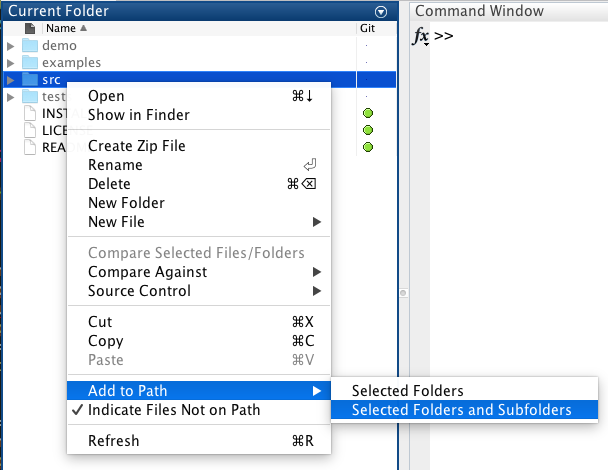
- If you plan to use an external solver, download and install it, and then add it to the Matlab path. If you have and intent to use
linprog(which we do not recommend given that it is not that robust), you don't need to do anything. - Run the
demo/demo_optimize_stock.mto check that everything is ok. If it outputs two figures, you're good to go. If it does not, make sure the solver selected is the right one.
For solver installation, you'll have to refer yourself to the solver documentation. Usually, this implies downloading the code, adding it to the Matlab path and setting a few environment variables (that's the annoying part).
A first example : Production Planning
This example can be run interactively using the demo/interactive_demo_optimize_stock.m file (just run this file and follow instructions in the Matlab prompt), or in a more classical way using the demo/demo_optimize_stock.m file.
This problem is the production planning under uncertainty problem. Assume we have a product that we can produce at time 1, and that we can sell at time 2. The main issue is that at time 2, the demand is uncertain.
To fix ideas, assume we produce, at time 1, \(x\) of our product, and that we sell \(s\) of it at time 2. \(C\) will denote the unit cost of production, \(P\) the sale price. \(d(\xi)\) is the (random) demand at time 2. Stated like that, at time 1, the problem is $$ NLDS(1) = \min_{x} C x $$ $$ x \geq 0 $$ while at time 2 we have $$ NLDS(2,\xi) = \min_{s} – P s $$ $$ s \geq 0 $$ $$ s \leq d(\xi) $$ $$ s \leq x $$
This formulation is the most important piece of information. It will be used to describe to the toolbox what problems need to be solved at each node. We can already notice a few key facts: at time 1, we only have variables from time 1 ; at time 2, we have variables from time 2, and the variables (solution) from time 1 can appear in the right-hand side of the constraints, linearly. Same for the random parameter, that can appear linearly in the right-hand side of the constraints.
Now let's turn ourself to the implementation of this problem.
The lattice
The lattice is what will be used to describe the evolution of the uncertainty, the number of scenarios, etc. In this problem, we will assume the random demand (at stage 2) \(d(\xi)\) can take two different values (low or high) with equal probability. At stage 1, we don't have any uncertainty. To represent that, we will use a scenario tree (a lattice), with one node at time 1 and 2 nodes at time 2. Assume we have defined the following demand function
function out = demand(t,i)
% We don't have any randomnes at stage 1, no we don't store anything
if t == 1
    out = [] ;
% At time 2, the demand is random, either 2 or 3, depending on the scenario:
else
    if i == 1
        out = 2 ;
    elseif i == 2
        out = 3 ;
    end
end
endH = 2 ;
nNodes = 2 ;
lattice = Lattice.latticeEasy(H, nNodes, @demand) ;latticeEasy is optional, and is used to store some information at each node of the scenario tree.
If provided, it should be a function of two arguments, the time t and the index of the node i. It can return anything you want,
and the data returned will be stored in the scenario tree, and available when building the NLDS problems.
To help visualise what the lattice is, the function plotLattice is quite useful.
In this case, it plots the following (the figure was slightly modified by hand)
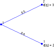
The numbers indicate the id of each of the node. We see that at stage 1, there is only one node, with equal probabilities (1/2) to go to each of the nodes of stage 2.
At stage 2, there are 2 nodes, where the random demand \(d(\xi)\) is either 2 or 3.
The variables
Now that the scenario tree has been created, we need to define the variables of our problem, namely \(x\) and \(s\). To do so, we simply type something like
x = sddpVar(1,1) ;
s = sddpVar(1,1) ;1,1 are optional (x = sddpVar() would have been just fine) but used to emphasize the fact that x and y are scalars.
The NLDS
Now, let’s turn to the core of the problem, the definition of the NLDS problems.
It will describe what needs to be solved at each stage.
The aim of this function is to return the constraints and the objective function at every stage.
Note that it is completey different whether scenario.time equals 1 or 2. In the second case, it will differ depending on the value
of the demand, stored in scenario.data.
function [cntr, obj] = nlds(scenario, x, s)
C = 1 ;
S = 2 ;
% It at stage 1, the problem is
% min C x + E(V(x))
% s.t. x >= 0
% So we write the following constraints :
% x >= 0
% and the objective function, without the E(V(x)) : the toolbox
% automatically takes care of that
% min C * x
if(scenario.time == 1)
% Constraint
cntr = x >= 0 ;
% Objective
obj = C * x ;
end
% If at stage 2, the problem is
% min - P s
% s.t. s >= 0
% s <= d(xi)
% s <= x
% (by default we minimize, so the '-' is needed)
if(scenario.time == 2)
% Constraints
pos = s >= 0 ;
notExceedDemand = s <= scenario.data ; % data is the random demand store into each node (scenario)
notExceedStock = s <= x ;
% Concatenate all constraints together
cntr = [notExceedDemand ; notExceedStock ; pos];
% The objective
obj = -S * s;
end
endEverything together
We can now put everything together, as shown by the following file. A few last things are needed in order to run SDDP. We first "compile" the lattice with the models
lattice = lattice.compileLattice(@(scenario)nlds(scenario,x,s)) ; nlds function one way or another. But you should not define
the variables inside nlds.
We then define a few parameters using the sddpSettings() function.
params = sddpSettings('algo.McCount',10, ...
'stop.iterationMax',10,...
'stop.pereiraCoef',0.1,...
'solver','linprog')help sddpSettings in the Matlab prompt. Important : you should set up the right value for solver. If you don't have Gurobi (gurobi) or Cplex (cplex), put Linprog (linprog) as a solver. We do recommend using gurobi or cplex if possible.
We finally call the sddp function using the compiled lattice and the parameters using
output = sddp(lattice,params);% DEMO OPTIMIZE STOCK
clc ; close all ; clear all ;
%% 1. Lattice creation
H = 2 ;
nNodes = 2 ;
lattice = Lattice.latticeEasy(H, nNodes, @demand) ;
figure ;
lattice.plotLattice(@(data) num2str(data)) ;
%% 2. Variables declaration
x = sddpVar(1,1) ;
s = sddpVar(1,1) ;
%% 3. NDLS declaration
lattice = lattice.compileLattice(@(scenario)nlds(scenario,x,s)) ;
%% 4. Run SDDP !
params = sddpSettings('algo.McCount',25, ...
'stop.iterationMax',10,...
'stop.pereiraCoef',2,...
'solver','linprog') ; % You need to adapt this for your solver.
output = sddp(lattice,params) ;
lattice = output.lattice ;
plotOutput(output) ;
%% 5. Finally, retreive the solution.
nForward = 10 ;
for i = 1:nForward
[~,~,~,solution] = forwardPass(lattice,'random',params) ;
xVal(i) = lattice.getPrimalSolution(x, solution) ;
sVal(i) = lattice.getPrimalSolution(s, solution) ;
end
disp('x') ;
disp(xVal) ;
disp('s') ;
disp(sVal) ;nlds passed to compileLattice should take exactly one argument, a scenario.
It is very important that the variables x and s are defined outside of the function. They should be the same between the
different calls to nlds so that the program can make the link between the different stages.
The last bit of code is used to retreive the optimal solution.
You can ignore it for now. But if you're curious, here's how it works : after completion of sddp, we
retreive the lattice and the cuts using lattice = output.lattice. We then do a series of forward pass
using the forwardPass function. Then, using the result, we assign to xVal and sVal the
numerical value using
xVal(i) = lattice.getPrimalSolution(x, solution) ;
sVal(i) = lattice.getPrimalSolution(s, solution) ;The output of the algorithm, displayed using
plotOutput(output)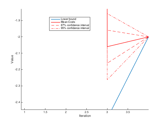
We see that at iteration 4, the algorithm has converged, since the lower-bound is equal to the (estimated) mean cost.