Installation

Basic installation instructions are available on the Quick Start page. For detailed information on solver installation, please refer to the solver installation instructions. Please remember to add the solver to the Matlab path before using FAST.

What can FAST solve ?

FAST can solve Multi-stage Stochastic Linear Programs. These problems can be described (for a reference, see for instance LINMA2491 notes from Anthony Papavasiliou at UCL) in general as $$ \min c^1 x^1 + \mathbb{E}_{\xi^2} [ \min c^2(\omega) x^2(\omega) + \mathbb{E}_{\xi^3} [ \min c^3(\omega) x^3(\omega) + \dots + \mathbb{E}_{\xi^H} \min c^H(\omega) x^H(\omega) ] \dots ] ] $$ subject to linear constraints of the form $$ W^1 x^1 \geq h^1 $$ $$ W^2 x^2(\omega^2) \geq h^2(\omega) - T^1(\omega^2) x^1 $$ $$ \cdots $$ $$ W^t x^t(\omega^t) \geq h^t(\omega) - T^{t-1}(\omega^t) x^{t-1}(\omega^{t-1})$$ $$ \dots $$ $$ W^H x^H(\omega^H) \geq h^H(\omega) - T^{H-1}(\omega^H) x^{H-1}(\omega^{H-1}) $$ $\omega^t$ refers to the randomness at time $t$ and $x^t(\omega^t)$ describes the (random) state of the system at time $t$. All superscripts indicate time. We can thus see that the type of equations we can solve are described by the following set of features:

At each time, the equations are linear
At each time, we can handle uncertainty in the right-hand side of the constraints
The solution from time $t-1$ ($x^{t-1}(\omega^{t-1})$) can also appear in the right-hand side at time $t$
Amongst the different scenarios $\omega^t$ at time $t$, all variables are the same, and the matrix in front of $x^t$ is constant amongst these scenarios. This is reflected in the fact that $W^t$ does not depend on $\omega^t$.

Note that this problem can formally be formulated as a huge linear problem. But it would be almost impossible to solve this problem using a black-box LP solver.

In order to describe such problems, it is useful to notice that we can completely capture them by defining a NLDS (Nested Linear Decomposition Subproblem). We then define $$ NLDS(t, \omega^t) : \min c^t(\omega^t) x^t(\omega^t) + V^t(x^t(\omega^t)) $$ $$ W^t x^t(\omega^t) \geq h^t(\omega^t) - T^{t-1}(\omega^t) x^{t-1} $$ where $V^t(x^t(\omega^t))$ captures the effect of the remaining stages, where $x^{t-1}$ is the fixed solution from the previous stages and where $\omega^t$ captures the uncertainty at stage $t$. This NLDS formulation is the central piece of information that you - the user - will need to supply FAST with in order to solve these problems.

The key idea of the SDDP algorithm - that FAST then leverage - is to solve nested NLDS, iteratively building a more and more accurate approximation of the $V^t(x^t)$ function.

In order to describe uncertainty, the SDDP algorithm uses a Lattice. This Lattice is a tree describing the propagation and evolution of uncertainty through time. At each time there are a certain number of nodes, connected to nodes at previous and next time, with transition probabilities.

Hydro Thermal Scheduling

The code of this problem can be found in the examples/hydro thermal folder.

This problem is the problem of Hydro Thermal Scheduling. The setup is the following : assume we have a dam and a thermal power plant. The dam can store a limited amount of water, which can then be used to produce free electricity. The only issue is that the amount of rainfall we observe at each period is random. On the other hand, the fuel power plant can produce electricity whenever we want, but it doesn't come for free. At each stage, we also have a known demand to satisfy.

Let's know try to put that into equations. Let's assume we will work over $H$ time-steps. We will denote by $x_t$ the water-level in the dam at time $t$. We will denote by $y_t$ the amount of water, stored in the dam, converted into electricity. And finally, we denote by $p_t$ the amount of power produced by the fuel power plant.

Let's denote by $C$ the marginal cost of the fuel, by $d$ the demand we need to satisfy at each time-step and by $V$ the maximum amount of water that can be stored in the dam. Finally, let's assume that at time $0$, the dam is empty, and denote by $r(\xi_t)$ the random amount of rain at stage $t$.

Considering all of this, at each stage, the problem can be stated as follows : $$ NLDS(t,\xi_t) : \min_{x_t,y_t,p_t} C p_t $$ subject to $$ x_t \leq V $$ $$ x_t \leq x_{t-1} + r(\xi_t) - y_t $$ $$ p_t + y_t \geq d $$ $$ x_t, y_t, p_y \geq 0 $$ In this problem, that $ x_{t-1} $ is considered fixed (as explained before)

There's a few things worth to be noted. First, note that the uncertainty only appears in the "right-hand side" of the problem. Uncertainty cannot appears in the coefficient matrix $W^t$ as stated before. Also note that only variables from this stage and the previous stage can appears (this is not a real limitation in practice).

In order to solve this problem with FAST we need to define the three main pieces of information:

A lattice, to describe transition probabilities and dependencies between stages.
The variables of the problems
The NLDS

Then, everything can be fairly easily combined together.

The Lattice

We thus need to describe the uncertainty in the problem. Let us say that, at each time, the random rain $d(\xi_t)$ can either be "low" ($d(\xi_t) = 2$) or "high" ($d(\xi_t)$ = 10). Assume we have defined the following function

function out = rainfall(t,i)
high = 10 ;
low = 2 ;
if t == 1
    out = (high + low)/2 ;
else
    if i == 1
        out = low ;
    else
        out = high ;
    end
end
end

that returns, at a time $t$ and for a node index $i$, the corresponding rainfall.

Now we define the lattice. We can easily define a lattice with uniform transition probabilities like that:

H = 5 ;
lattice = Lattice.latticeEasy(H, 2, @rainfall) ;

where we use $H = 5$, and where at each stage we have two possibles scenarios. In this case, the rainfall function will be called at every node of the lattice, and the result will be available during the NLDS definition (see below).

Finally, we can also visualize this lattice using

figure ;
lattice.plotLattice(@(data) num2str(data)) ;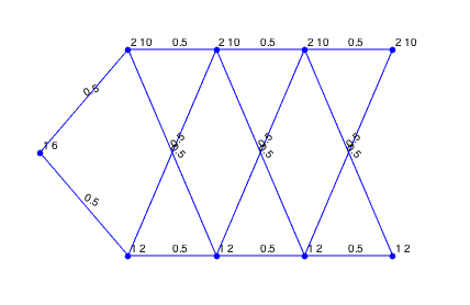

And we obtain

Note that the latticeEasy function always assumes only one scenario (node) at time $t = 1$.

The Variables

We now need to define the variables that we will use to describe the NLDS at every stage. Note the following:

We need to have the sames variables across all scenarios at a given stage
We need to define the variables only once. To do so, the idea is to declare the variables outside SDDP, and then pass the variables to the function that will be used to build the NLDS problems (see below)

In our example, we want to have variables $x_t, y_t, p_t$, so 3 variables at each stage. To do so, we thus simply create the variables like that (we store all variables in a struct var)

var.x = sddpVar(H) ; % The reservoir level at time t
var.y = sddpVar(H) ; % For how much we use the water at time t
var.p = sddpVar(H) ; % For how much we use the fuel generator at time t

So note that we do not declare different variables for the different scenarios, just for the different stages.

In this case we thus define the variables using the sddpVar function. This function can take an arbitrary number of argument, and will thus create an array of sddpVar objects. If needed, if we have say $L$ variables $x$ at each time, we could define

x = sddpVar(L, K) ;

so that at each stage, we would have multiple variables of the same "type" $x$.

The NLDS

Now that the variables have been declared, we need to build, at each stage and node, the NLDS problems (without the $V^t(x^t)$ term). To do so, we need to create a function that takes as input a scenario object, and return, at each node, the objective $c^t(\omega)x^t(\omega)$ and the constraints $W^t x^t(\omega^t) \geq h^t(\omega^t) - T^{t-1}(\omega^t) x^{t-1} $.

For instance in our case, we define the following function

function [cntr, obj] = nlds(scenario, var)

t = scenario.getTime() ;

C = 5 ;
V = 8 ;
d = 6 ;

x = var.x ;
y = var.y ;
p = var.p ;

% Fuel cost
fuel_cost = C * p(t) ;
% Maximum reservoir level
reservoir_max_level = x(t) <= V ;
% Meet demand
meet_demand = p(t) + y(t) >= d ;
% Positivity
positivity = [x(t) >= 0, y(t) >= 0, p(t) >= 0] ;
% Take rain into account
if t == 1
    reservoir_level = x(1) + y(1) <= scenario.data ;
else
    reservoir_level = x(t) - x(t-1) + y(t) <= scenario.data ;
end

obj = fuel_cost ;
cntr = [reservoir_max_level, ...
        meet_demand, ...
        positivity, ...
        reservoir_level] ;
end

where all the variables are passed using the structure var.

Building constraints and objective function is fairly intuitive. Basically, instructions like

fuel_cost = C * p(t)

creates a variable fuel_cost that is an affine expression, in this case just equal to $C p_t$. And instructions like

reservoir_level = x(t) - x(t-1) + y(t) <= scenario.data ;

defines a linear inequality constraint equivalent - without surprise - to $x_t - x_{t-1} + y_t \leq d(\xi_t)$. Note that we actually use $x_{t-1}$ as permitted, but we can't use $x_{t-2}, x_{t-3},\dots$.

Note that in this code, we use the scenario.data concept. scenario.data contains the output of the rainfall function, that was passed to the latticeEasy function. It thus contains, at each node $(t, i)$, the output of the rainfall function, i.e., the amount of rain at this scenario (node).

We finally return both the constraints and the objective function. All constraints are simply concatenated into a single variable cntr then returned.

Once we have defined the nlds function, we pass this function to the compileLattice function that will build, on top of the lattice, all the NLDS models

lattice = compileLattice(lattice,@(scenario)nlds(scenario,var),params) ;

We clearly see here that the variables are passed to the nlds function, but are not defined inside it. This is the same mechanism as the one explained here.

Everything together

Once we have defined the nlds function, the whole code looks like the following

clc ; close all ; clear all ;
H = 5 ;
% Creating a simple 5 stages lattice with 2 nodes at second stage
lattice = Lattice.latticeEasy(H, 2, @rainfall) ;
% Visualisation
figure ;
lattice.plotLattice(@(data) num2str(data)) ;
% Run SDDP
params = sddpSettings('algo.McCount',25, ...
                      'stop.iterationMax',10,...                      
                      'stop.pereiraCoef',2,...
                      'solver','linprog') ;
var.x = sddpVar(H) ; % The reservoir level at time t
var.y = sddpVar(H) ; % For how much we use the water at time t
var.p = sddpVar(H) ; % For how much we use the fuel generator at time t                  
lattice = compileLattice(lattice,@(scenario)nlds(scenario,var),params) ;                                    
output = sddp(lattice,params) ;

% Visualise output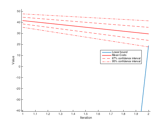
plotOutput(output) ;

In addition of defining the lattice, the variables and the nlds function, a few settings can be set. These are discussed in the next section. Note, however, the 'solver','linprog' parameter. If you are using another solver (we recommand gurobi or cplex), you need to change this setting using either 'gurobi', 'mosek', 'cplex' or 'glpk'. Again, do not forget to add your solver to the Matlab path. The plotOutput function can be used to see the evolution of the lower-bound and the mean cost estimates (see below). It returns the following hydro_convergence

Parameters

So far, we haven't really modified any parameter. But FAST allows you to change most of the algorithm parameters to tune them for your problem. To do so, it is required to build a parameter structure using the sddpSettings function, like

params = sddpSettings('algo.McCount',10, ...
                      'solver','gurobi') ;

This function takes pairs of string-value. For more information on each option (including their default value), type help sddpSetting in the matlab prompt.

For instance, one can pass parameters to the solver using the solverOpts field like this

params = sddpSettings('solverOpts',struct('maxIter', 10)) ;

Doing so require to understand the solver behaviour, so we advise you to read the solver documentation first.

Convergence criterion

As a first basic termination criterion, there are

params = sddpSettings('stop.iterationMin',5,...
                      'stop.iterationMax',20) ;

which is self-explanatory.

Classical termination criterion

In this section we focus on convergence parameters. Roughly speaking, the standard convergence criterion for SDDP is the following: the algorithm stops at iteration $i$ if the lower-bound $L_b$ and the mean-cost $\mu_C$ are such that $$ L_b \geq \mu_C - c \frac{\sigma_C}{\sqrt{K}} $$ where $K$ is the number of Monte-Carlo trials and $\sigma_C$ is the standard deviation of the cost. Finally, $c$ is a parameter controlling the size of the required confidence interval. This criterion follows directly from the central limit theorem.

By default, FAST will use this termination criterion with $c = 2$ corresponding to a standard 95% confidence interval. This value can be changed by setting for instance

params = sddpSettings('stop.pereiraCoef',0.1) ;

which will set $c = 0.1$. We can also change the number of Monte-Carlo samples and the maximum number of iterations

params = sddpSettings('stop.pereiraCoef',0.1,...
                      'algo.McCount',200,...
                      'stop.iterationMax',20,...) ;

A remaining question of importance is the following : how to choose $K$ ? A simple criterion to be used can be the following. Assume we use $c = 2$, and say we want the confidence interval to be a fraction $\beta$ of the mean cost $\mu$. Let $\sigma$ be an estimate of the standard deviation of the cost at convergence. We can thus solve $$ \frac{\frac{2\sigma}{\sqrt{K}}}{\mu} = \beta \Rightarrow K = \left( \frac{2 \sigma}{\beta \mu} \right)^2. $$ If we want say $\beta = 1\%$ we then have $$ K = 40000 \left( \frac{\sigma}{\mu} \right)^2. $$ Not surprisingly, the number of samples increases quadraticly with the ratio between the standard deviation and the mean cost.

Small standard deviation

In addition of this classical convergence criterion, in some case we may want to stop only when the standard deviation of the mean cost is small enough with respect to the lower bound. This translate into another termination criterion to meet: $$ \frac{\sigma_C}{\sqrt{K}} \leq \gamma |L_b| $$ where $\gamma$ is some parameter, than can be set using

params = sddpSettings('stop.stdMcCoef',0.1) ;

Note that by default, this termination criterion is not used.

Which criterion to choose ?

By default, the first termination criterion with say $c = 2$ should be enough. In order to choose which criterion to use, we need to set the stop.stopWhen field to one of these 4 values

params = sddpSettings('stop.stopWhen','pereira') ;

params = sddpSettings('stop.stopWhen','std') ;

params = sddpSettings('stop.stopWhen','pereira and std') ;

params = sddpSettings('stop.stopWhen','never') ;

The 4 options are pretty clear. Note that the last one mean we will stop at the maximum number of iteration. In practice, the first termination criterion should be good enough.

Accurate estimators of the mean

The problem with the standard approach is that we compute estimates of the mean cost with usually a small ($K$) number of samples. The algorithm actually allows for computation of an accurate mean every other iterations. To do so, we need the following options

params = sddpSettings('precise.compute',true,...
                      'precise.iterationStep',10,...
                      'precise.count',200,...) ;

This will compute every $10$ iterations an accurate estimator of the mean using $200$ Monte Carlo samples. It will be displayed in the Matlab prompt.

Precise and regular convergence

The problem with the standard convergence criterion is that we check convergence criterion with what is usually a small number of sample ($K$). Another approach would be to use a small number of samples to build the cuts ans to use a larger number of sample, every other iteration, to check convergence (like we do above to have an accurate estimator of the mean). This is the idea behind the stop.regular and stop.precise fields. If stop.regular is set to false, then the algorithm will not check convergence during the standard iteration ; otherwise it will. If the stop.precise is set to true, however, it will also check convergence criterion using the precise estimate (see above). So in short, to check convergence with only the precise estimate, we should use the options

params = sddpSettings('stop.regular',false,...
                      'stop.precise',true,...
                      'precise.compute',true,...
                      'precise.iterationStep',10,...
                      'precise.count',200,...) ;

Interpreting the Output

FAST outputs quite a few information when run with the ('verbose',1) default parameter. It also outputs, at the very end, a structure with a number of fields that can be used to analyze the solution. Broadly speaking, there are three types of outputs:

Startup information : at the very beginning, when the algorithm is started, it essentially displays a few warning and technical stuff, and then by default it prints all the parameters passed to the algorithm. It can be useful to quickly check that all the parameters are the right ones, but otherwise, you can mostly ignore this.

Convergence information : this is the most important part. During the execution of the algorithm, at every step, it displays something like

-------------
Iteration 1
-------------
LowerBound                                 : 5.060000e+05
Mean(ForwardCosts)   (K =  20)             : 1.068810e+07
Std(ForwardCosts)    (K =  20)             : 1.624004e+05
95 pc confidence interval around mean cost : [1.061547e+07   1.076073e+07]
95 pc confidence interval for solution     : [5.060000e+05   1.076073e+07]
Confidence interval desired (coef 1.0e-01) : [1.068447e+07   1.069173e+07]
Pereira's  criterion (    to be checked)   : not met
StdMc      criterion (not to be checked)   : not met
This iteration took 12.383474 s.

The LowerBound fields gives the value of the $L_b$ parameter, Mean(ForwardCost) the value of $\mu_C$ and Std(ForwardCost) the value of $\sigma_C$. The fourth and fifth fields are, respectively, $ \mu_C \pm \frac{2\sigma_C}{\sqrt{K}} $ and $ [L_b, \mu_C + \frac{2\sigma_C}{\sqrt{K}}] $. Finally, we then have $ \mu_C \pm \frac{c\sigma_C}{\sqrt{K}} $. The next fields are pretty self-explanatory.

Output structure : the sddp function returns a structure as the output. This structure, say output, has the following structure
```
>> output

output =

       solution: {HxK cell}
        lattice: [1x1 Lattice]
    lowerBounds: [Ix1 double]
       meanCost: [Ix1 double]
           stds: [Ix1 double]
    runningTime: time
         params: [1x1 struct]
                
```
where we have used H to denote the number of stages, K for $K$ and I for the number of iterations. The solution field is a cell array containing, for each Monte-Carlo sample of the last iteration, the solution at each of the node selected. lattice contains the compiled lattice with the cuts (see next section on how to use that). lowerBounds, meanCost and stds contain, respectively, the values of $L_b$, $\mu_C$ and $\sigma_C$ for all iterations. Finally, runningTime and params contain respectively the running time (in seconds) of the algorithm and the parameters used (exactly the same as the input parameters).

Forward Passes

Once the SDDP algorithm has terminated, it is possible to do "forward passes" on the lattice, now containing cuts. This allows for the retrieval of "optimal" values for the variables. In the Hydro-Thermal Scheduling problem, this can be down using this piece of code

% Forward passes
lattice = output.lattice ;
nForward = 5 ;
objVec = zeros(nForward,1);
x = zeros(nForward,H);
y = zeros(nForward,H);
p = zeros(nForward,H);
dataForward = cell(nForward,1) ;
for  i = 1:nForward
    [objVec(i),~,~,solution] = forwardPass(lattice,'random',params) ;    
    x(i,:) = lattice.getPrimalSolution(var.x, solution) ;
    y(i,:) = lattice.getPrimalSolution(var.y, solution) ;
    p(i,:) = lattice.getPrimalSolution(var.p, solution) ;
    dataForward{i} = lattice.getDataSolution(solution) ;
end

In this code, we do 5 forward passes. At each step, we get a objective value and we can retreive the solution (in term of the variables $x, y, p$) using the lattice.getPrimalSolution function, as well as the path and the realisation of the random variable using lattice.getDataSolution. The node index and the realisation of the random variable at stage $t$ are accessible via the fields dataForward{i}.path(t) and dataForward{i}.data{t}.

These functions (methods of the Lattice class) have to be applied on the outputted lattice (hence the lattice = output.lattice ; code), and takes as input the variables (for lattice.getPrimalSolution) and the solution structure from the forwardPass function.

In addition, note that, technically, forward passes do not require the use of an "outputted" lattice with cuts. Forward passes can be applied simply on a compiled lattice with NLDS. This can be useful in order to test other heuristic policies for instance.

More on the Modeling

The modeling part of the toolbox is used to define the variables, the (linear) objective and (linear) constraints in the NLDS formulation.

Variables

Variables are declared using the sddpVar functions, using either this syntax

x = sddpVar(n1, n2, n3, ..., nk)

x = sddpVar([n1 n2 ... nk])

Both syntaxes (and, actually, any combination of both) will create an array of size $n_1 \times n_2 \times \cdots \times n_k$ filled with independent variables (actually, affine expressions of the shape $1\cdot x + 0$). Such an array is a classical Matlab array and can then be used as usual, i.e., for instance we can extract individual columns

>> x = sddpVar(1, 4, 2)

x = 

1x4x2 array of affine expressions
>> y = x(:, 1:2, 1)

y = 

1x2 array of affine expressions

We can also create affine expression. For instance, this

>> x = sddpVar(5)

x = 

5x1 array of affine expressions
>> sumx = sum(x)

sumx = 

1x1 array of affine expressions

creates a variable sumx defined as the sum of the variables in x.

Objective

Once the variables have been created, defining the objective can be done very naturally, using operations like *, sum, +, -, etc. For instance,

x = sddpVar(5) ; y = sddpVar(3) ; obj = sum(x) + [1 2 3]*y 

obj = 

1x1 array of affine expressions

creates an objective function like $$ obj = x_1 + x_2 + x_3 + x_4 + x_5 + y_1 + 2 y_2 + 3 y_3. $$

Constraints

Now that we can define affine expressions, constraints can be done by using the >=, <=, = operators between arrays of affine expression of the same size. For instance,

>> x = sddpVar(3, 2) ; y = sddpVar(3, 2) ; cntr = [x + 2*y >= rand(3, 2)] 

cntr = 

1x1 array of >= constraint of size 3x2

creates an inequality contraint between arrays of size $3 \times 2$.

Constraints defined like that can then be concatenated and returned as a single constraints array, like it is done in the nlds function.

Pre-Cutting the Lattice

Sometimes, it is useful to be able to "precut" the lattice using the result of some heuristic policy. Basically, this is equivalent of using a feasible forward solution, and running a backward pass on it. This can be done using the precut function. For instance, if we want to test a policy where $x_1 = 2, x_2 = 3$ (and in which we actually don't care about the value of $s_1$ and $s_2$ since they do not appear in any right-hand side as "trials") we can use

x = sddpVar(2) ; 
s = sddpVar(2) ; 
% (...)
lattice = precut(lattice, [x ; s], [2 ; 3 ; nan ; nan], params) ;

This function will fix $x_1$ and $x_2$ when they appear as right-hand sides, will generate the cuts, and return the new "precut" lattice. Note that since $s_1$ and $s_2$ do not appear as trials in any right-hand side, their value is unrelevant, and we use nan. Note that we still need to include all variables of the problem in the precut function.

Retrieving the Cuts

Given the lattice outputted by SDDP, we can also retreive the cuts. Internally, cuts are expressed as $$ \theta \geq e - E x $$ where $e \in \mathbb{R}^k$ and $E \in \mathbb{R}^{k \times n}$ if we have $k$ cuts and $n$ variables.

To retreive $E$ and $e$, it is sufficient to call

[cutCoeffs, cutRHS] = lattice.getCuts(t, n, [x y z]) ;

if we want to retreive the cuts at time t, node n and if the variables are this node are exactly [x y z]. Note that the order in which the variables are provided do not matter, but all the variables at this node should be present (and nothing more). The column of $E$ will be such that the order match the order of the variables provided.

Given $E$ and $e$, it is even possible to plot the cuts. For instance, if we only had two variables $x_1$ and $x_2$, to plot the cuts at $t = 1$ and $n = 1$, we can use

x = sddpVar(2) ;
% (...) Rest of the code
output = sddp(lattice, params) ;
lattice = output.lattice ;
% Getting cuts
[cutCoeffs, cutRHS] = lattice.getCuts(1, 1, x) ;
% x contains two variables, x1 and x2
[x1, x2] = meshgrid(0:0.1:5, 0:0.1:5) ;
vx = zeros(size(x1)) ;
for i = 1:size(x1, 1)
    for j = 1:size(x1, 2)
        vxall = cutRHS - cutCoeffs * [x1(i,j) ; x2(i,j)] ;
        vx(i,j) = max(vxall) ;
    end
end
figure ;
surf(x1, x2, vx) ;

which will plot the cuts in the space $(x_1,x_2) \in [0,5]\times [0,5]$.

Lower-Bound on Theta

An important parameter of the algorithm is the initial lower-bound on $\theta$, which is basically a lower-bound for the value function $V^t$ at each stage. This is only used to prevent unboundedness in the solvers. If your problem has strong negative value function, you may want to decrease this value by setting the parameter

params = sddpSettings('algo.minTheta',-1e6)

to a more negative value. The default value is $-10^{-3}$ (which is completely arbitrary in some sense).

Links and Resources

Operations Research (LINMA 2491) class at Université catholique de Louvain from Anthony Papavasiliou
Poster on FAST presented at the ICME Xpo Event (May 20, Stanford)
M.V.F. Pereira and L.M.V. G Pinto, Multi-stage stochastic optimization applied to energy planning, Mathematical Programming, 52 (1991), 359-375.