Lecture 16: Statistical Significance#
STATS60 so far#
Unit 1 – Thinking About Scale:
Putting numbers in context, Fermi estimates, cost benefit analysis.
Unit 2 – Exploratory Data Analysis:
Terminology, data visualization, data summaries.
Unit 3 – Probability:
Computing probabilities, conditional probability, probability fallacies, expectation.
Looking ahead#
Unit 4 – Estimates, hypothesis testing and experiments:
Generalizing from data to a larger group.
Today:
Significance: how strong is the evidence?
Chimpanzees problem-solving.
Significance#
Organ donations#
The wording of the question seems to have an impact on the proportion of people who sign-up to be organ donors.
Is the difference between groups large enough to statistically significant?
Statistical significance#
Statistically significant means that the results are unlikely to have occurred by random chance alone.
Example: it is possible that the different sign-up rates are due to chance, but this seems unlikely based on the study results.
Statistical significance asks “is our result unlikely to happen by random chance?”
To answer this, we will investigate what the results would like if any differences were due to random chance.
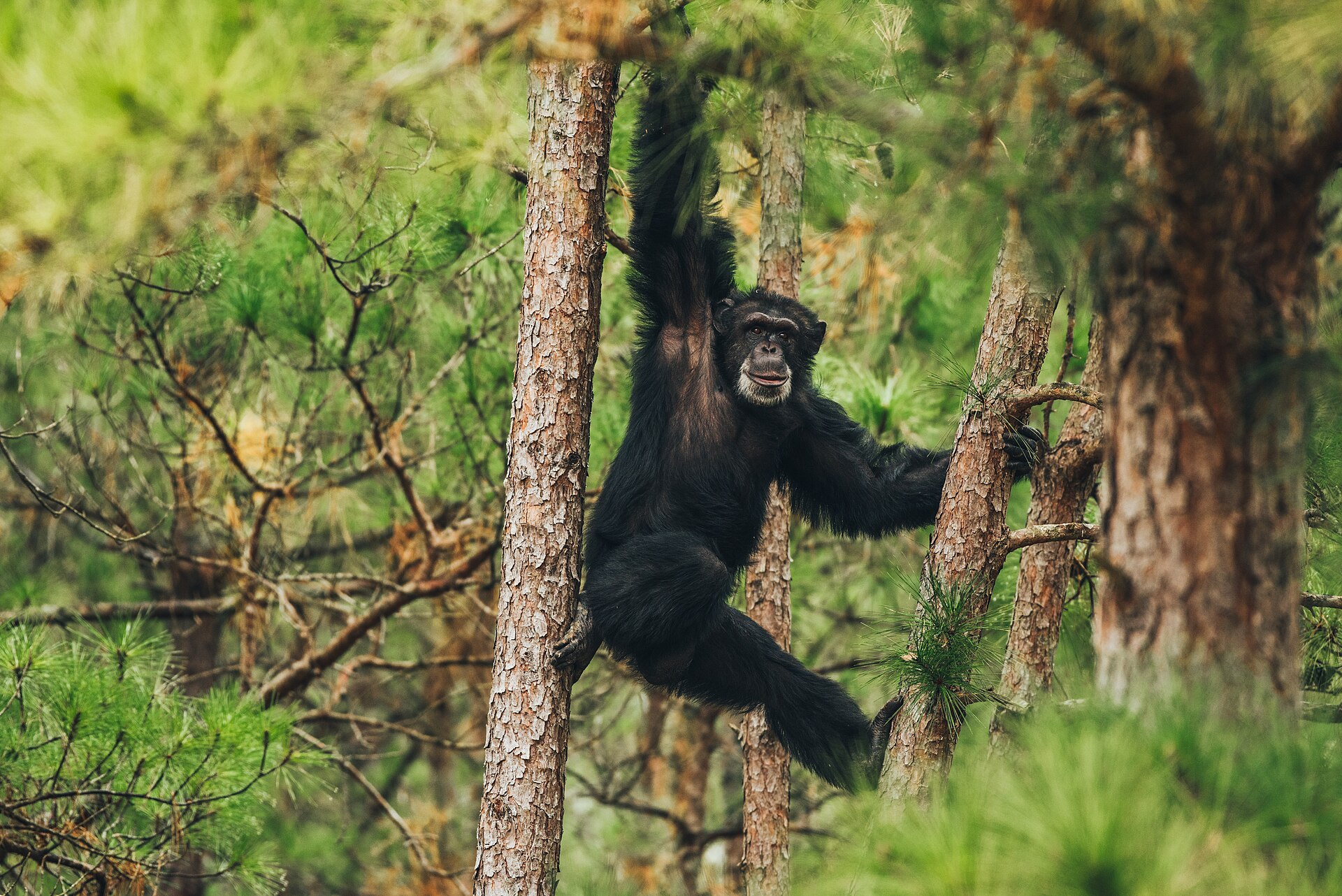
Chimpanzees and problem-solving#
Can chimpanzees solve problems?#
Chimpanzees are known to use tools and demonstrate simple problem-solving.
Premack and Woodruff (1978) wanted to know if chimpanzees could understand problems faced by people.
Sarah#
Sarah (an adult chimpanzee) was shown 8 videos of a human facing a problem.
Sarah was shown two photos where one photo has the correct solution.
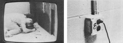
One of the problems and its solution. Sarah picked the correct photo 7 out of 8 times.
Observational units and variables#
In the chimpanzee problem-solving study:
a. What are the observational units?
b. What are the relevant variables?
a. The observational units are the problems.
b. A relevant variable is whether Sarah chose the correct picture.
Samples and statistics#
Definitions#
The set of observational units on which data is collected is called the sample.
The number of observational units in the sample is the sample size.
A statistic is a number summarizing the data in the sample.
Samples and statistics#
In the chimpanzee problem-solving study:
a. What is the sample size?
b. What would be a relevant statistic?
a. The sample size is 8 (the number of problems).
b. A relevant statistic is the proportion of times Sarah picked the correct picture (7 out of 8 times).
Beyond the sample#
Sample as a snapshot#
The 8 problems that were shown to Sarah are just a snapshot of Sarah’s ability to solve problems.
Sarah’s problem-solving can be thought of as a random process.
We want to know the long run probability of Sarah correctly answering a question.
Parameters#
Definition#
For a random process, a parameter is a long-run numerical property of the process.
Parameters are often written using Greek letters.
Example: the long-run frequency of Sarah correctly solving a problem. We will call this number \(\pi\) (a Greek p).
We won’t know the exact value of \(\pi\), but we can use a sample to make conclusions about the likely values \(\pi\).
Two explanations#
Sarah selected the correct photo in 7/8 attempts.
What are two possible explanations for why Sarah got 7 out of 8 correct?
a. Sarah knows how to solve problems and is using this skill to select the photo (the probability of correctly selecting the correct photo is larger than 0.5).
b. Sarah is just guessing (the probability of correctly selecting the correct photo is 0.50) and she got lucky in these 8 problems.
Which of these two explanations do you think is more a reasonable explanation? How would you convince a skeptic?
Tactile simulation#
How can we model what the study would have looked like if Sarah was just guessing?
Flip your coin 8 times and record the number of “heads” which we will call a success.

Questions#
Based on the histogram of results:
What does each square represent?
What was the most common outcome for number of heads in 8 coin tosses? Does that make sense?
Why did we need everyone to toss their coin 8 times? Why couldn’t we just ask one person and look at their results?
Where does Sarah’s observed result of 7 correct out of 8 fall in this histogram? Does “just guessing” seem to be a good explanation for 7 correct?
One proportion applet#
Instead of flipping more and more coins, we will use the One Proportion applet.
What value should we use for “probability of heads”?
What about “Number of tosses”?
If we draw many samples, what does each dot in the dotplot represent?
One proportion applet#
Based on the dotplot, how would you describe the result of 7 out of eight heads? Why?
a. Very surprising. b. Somewhat surprising. c. Not surprising.
It seems somewhat surprising because the 7 heads out of 8 tosses seems far out in the tail, and therefore unusual to happen by chance alone.
Quantifying surprise#
To quantify “how surprising” or “how unlikely” the observed result is, we need to calculate what proportion of times the simulation results were at least as surprising as the observed result.
In the One Proportion applet, we can use “Count samples” to find the number of times we got a result as extreme as 7 out of 8 heads.
What is the proportion of repetitions as extreme as our observed result?
p-values#
p-value#
The previous quantity (“proportion of as extreme repetitions”) is called a p-value.
Definition (p-value)#
A p-value is the probability of finding a result at least as extreme/surprising, in settings identical to the actual study, if outcomes happened by random chance alone.
A p-value is always between 0 and 1.
p-value example#
In the Chimpanzee study:
Settings identical to the actual study → 8 trials.
Random chance alone → probability of success is 0.5.
p-value visualization#
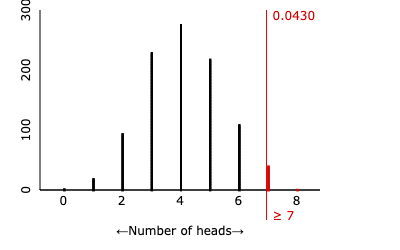
The p-value is represented by the red area in the dotplot.
The p-value is the tail area of the dotplot starting at 7, the number of correct answers in the study.
Simulations that resulted in 8 heads are also included.
p-value interpretation#
If Sarah was just randomly guessing, we would observe at least seven correct problems about 4.3% of the time.
If you used the applet on your own, would you get the same p-value? Will the p-value be close?
Null and alternative hypotheses#
Two possible explanations#
There were two potential explanation for why Sarah picked the correct photo in 7 out of 8 scenarios:
a. For any problem, Sarah tends to randomly pick one of the two photos.
b. For any problem, Sarah tends to pick the correct photo.
These potential explanations are called hypotheses.
Null hypothesis#
The first explanation (Sarah tends to pick randomly) is called the null hypothesis and is abbreviated as \(H_0\).
The null hypothesis corresponds to “just chance” or “no effect.”
Recall that \(\pi\) is the long-run frequency of Sarah selecting the correct photo.
Write the null hypothesis in terms of the parameter \(\pi\):
\(H_0 : \pi = 0.5\)
Alternative hypothesis#
The second explanation (Sarah tends to pick the correct photo) is called the alternative hypothesis and is abbreviated as \(H_A\).
The alternative hypothesis corresponds to “better than chance” or “an effect.”
Write the alternative hypothesis in terms of the parameter \(\pi\):
\(H_A : \pi > 0.5\)
p-values and hypothesis#
p-value is “small” → Evidence against \(H_0\) → Evidence for \(H_A\).
p-value is “not small” → No evidence against \(H_0\) → No evidence for \(H_A\).
Smaller p-value → Stronger evidence against \(H_0\) → Stronger evidence for \(H_A\).
p-value thresholds#
0.10 < p-value → Not much evidence against \(H_0\).
0.05 < p-value < 0.10 → Moderate evidence against \(H_0\).
0.01 < p-value < 0.05 → Strong evidence against \(H_0\).
p-value < 0.01 → Very strong evidence against \(H_0\).
You do not need to memorize these thresholds. You do need to remember:
Smaller p-value → Stronger evidence against \(H_0\).
Study conclusions#
The conclusions from the study can be stated in terms of the p-value and the null and alternative hypothesis:
The p-value (which is about 0.043) provides evidence against the null hypothesis, and evidence for the alternative hypothesis.
Thus, Sarah’s data provide evidence that, in general, for any similar problems, Sarah would tend to select the correct photo.
Going beyond the study#
Based on Premack and Woodruff (1978) do you have any questions related to chimpanzees’ abilities to solve problems?
Summary - samples and parameters#
Statistically significant means that the results are unlikely to have occurred by random chance alone.
The set of observational units on which data is collected is called the sample.
A statistic is a number summarizing the data in the sample.
For a random process, a parameter is a long-run numerical property of the process.
Summary - p-values and hypotheses#
A p-value is the probability of finding a result at least as extreme/surprising, if outcomes happened by random chance alone.
The null hypothesis corresponds to “just chance” or “no effect.”
The alternative hypothesis corresponds to “better than chance” or “an effect.”
Small p-value → evidence against the null hypothesis → evidence for the alternative hypothesis → data is statistically significant.
Computing p-values#
To compute a p-value, we need a model for what the results would have looked like if there was no effect.
Example: flipping a fair coin, using an applet.
Next, we repeat or simulate the results many times (1,000 is usually enough).
Finally, we compute the number of times the simulation was at least as extreme as the results we actually observed.
Computing p-values#
Looking ahead#
In different studies the details will be different:
Different setting (e.g. different number of trails).
Different statistic (e.g. a mean instead of a proportion).
Different model for “no effect” (e.g. 1/3 instead of 1/2).
But the core idea is the same:
To determine statistical significance: compare the observed data to what we would happen if there was no effect.
Can dogs detect COVID?#
Study background#
Dogs have a remarkable sense of smell.
Dogs can detect drugs, help with search and rescue and identify explosives.
A 2020 study investigated whether dogs can detect COVID-19.
Study background#
The dog would smell 4 sweat samples.
One sample was from a COVID positive person.
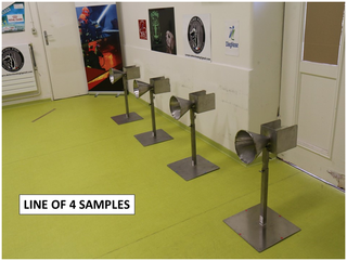
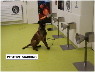
The dog was trained to mark the positive sample.
The dog marked the sample by sitting in front of it.
Study results#
One of the dogs was a Belgian Malinois Shepherd named Maika.
Maika correctly marked the covid positive sample in 32 out 38 trials.
What are two explanations for Maika’s results?
One proportion applet#
We can compute a p-value based on Maika’s result.
This time we will go straight to the One Proportion applet.
What value should we use for “probability of heads”?
What about “Number of tosses”?
p-value#
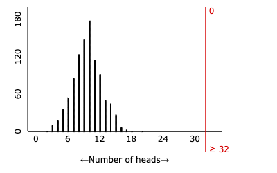
None of the simulated experiments results in a result as extreme as 32 out 38 heads.
We have very strong evidence against the null hypothesis.