Lecture 28: Outro#
STATS 60 / STATS 160 / PSYCH 10
Announcements
Review sessions
Skyler: Thursday 1:00 – 2:30 pm in CoDA E401
Michael: Friday 11:00 am – 12:00 pm in CoDA B40
Today’s lecture#
Overview of the quarter
Three themes for the class
What’s next if you’re stats-curious?
Remembering our journey#
Unit 1: Thinking about scale#
Numbers in statistics#
In statistics and data science, numbers are used to
Describe observations
Quantify how confident we are
But, Numbers are only meaningful in context.
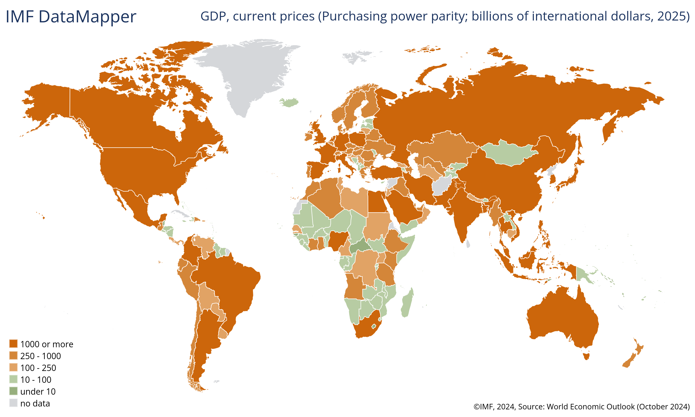
Is $10 billion a lot of money?

Three questions#
What type of number is this?
What can I compare this number to? Is it large or small compared to other similar values?
What would I have expected this number to be?
Ballpark estimates#
Set up a simple model to compute the quantity approximately by break up the estimate into small parts
How many visitors go on tours at Stanford per year?
\[\frac{\text{# visitors}}{\text{year}} = \frac{\text{# days}}{\text{year}} \times \frac{\text{# tours}}{\text{day}} \times \frac{\text{# visitors}}{\text{day}}\]
Approximate parts up to a factor of 10
Cost benefit analysis#
Ballpark estimates can be used to make important decisions.


Unit 2: Exploratory data analysis#
Putting data in context#
It is hard to find insight from looking at raw data.
Data visualization and data summaries let us choose what to communicate and focus on.
Data visualization#
Common graphic representations:
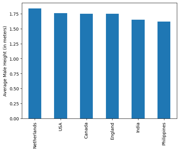
Bar chart and pie chart (categorical variables)
Time series (seeing how a variable changes over time)
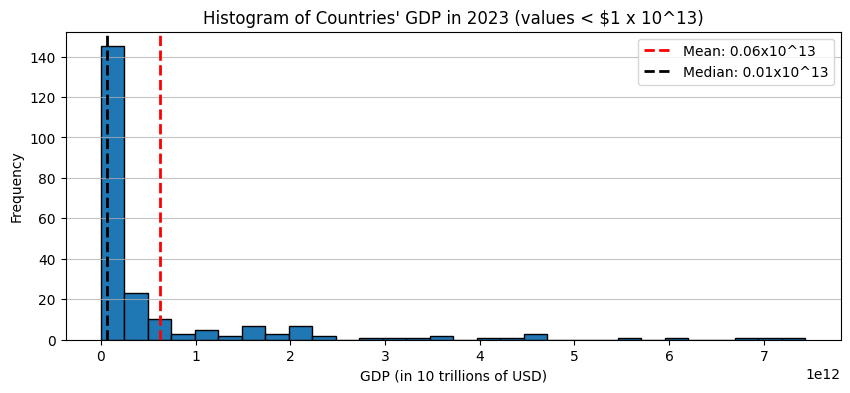
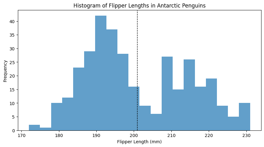
Histogram (one quantitative variable)
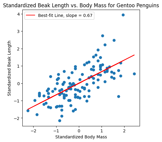
Scatter plot (two quantitative variables).
Effective data visualization#
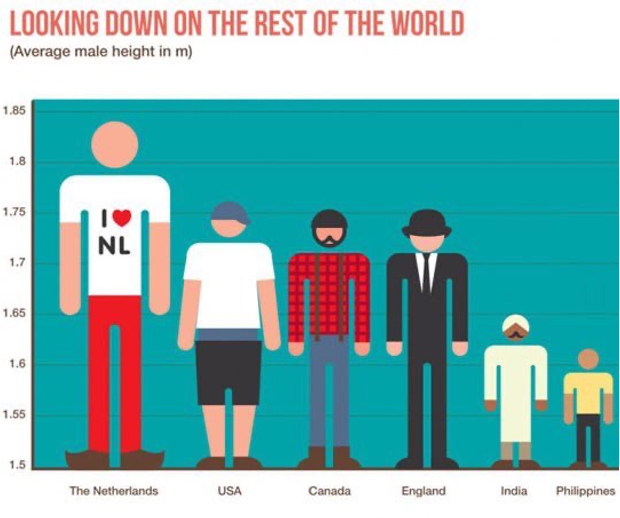
Deceptive data visualization#
Watch out for misleading data visualizations.
Summaries of center and variability#
Summaries of center: what is the one number that best summarizes the data?
Mean, median, mode.
Variability: how similar are the different datapoints in the dataset?
Would you rather be given \(\$150\) or flip a coin for \(\$300\)?
Variance, standard deviation, quantiles and gaps between quantiles.
Correlation and correlation coefficient#
What is the direction and strength of the association between two quantitative variables?
Misleading means#
The usefulness of a summary statistic depends on the data!
Outliers/skew
Multi-modal data
Subgroups
Unit 3: Probability#
Probability#
The mathematics of uncertainty.
One of the foundations of statistics.
Probability helped us:
Assess how likely/unlikely coincidences are.
Update our beliefs based on new information (conditional probability).
Generalize findings from data to a broader group of people (hypothesis testing and confidence intervals).
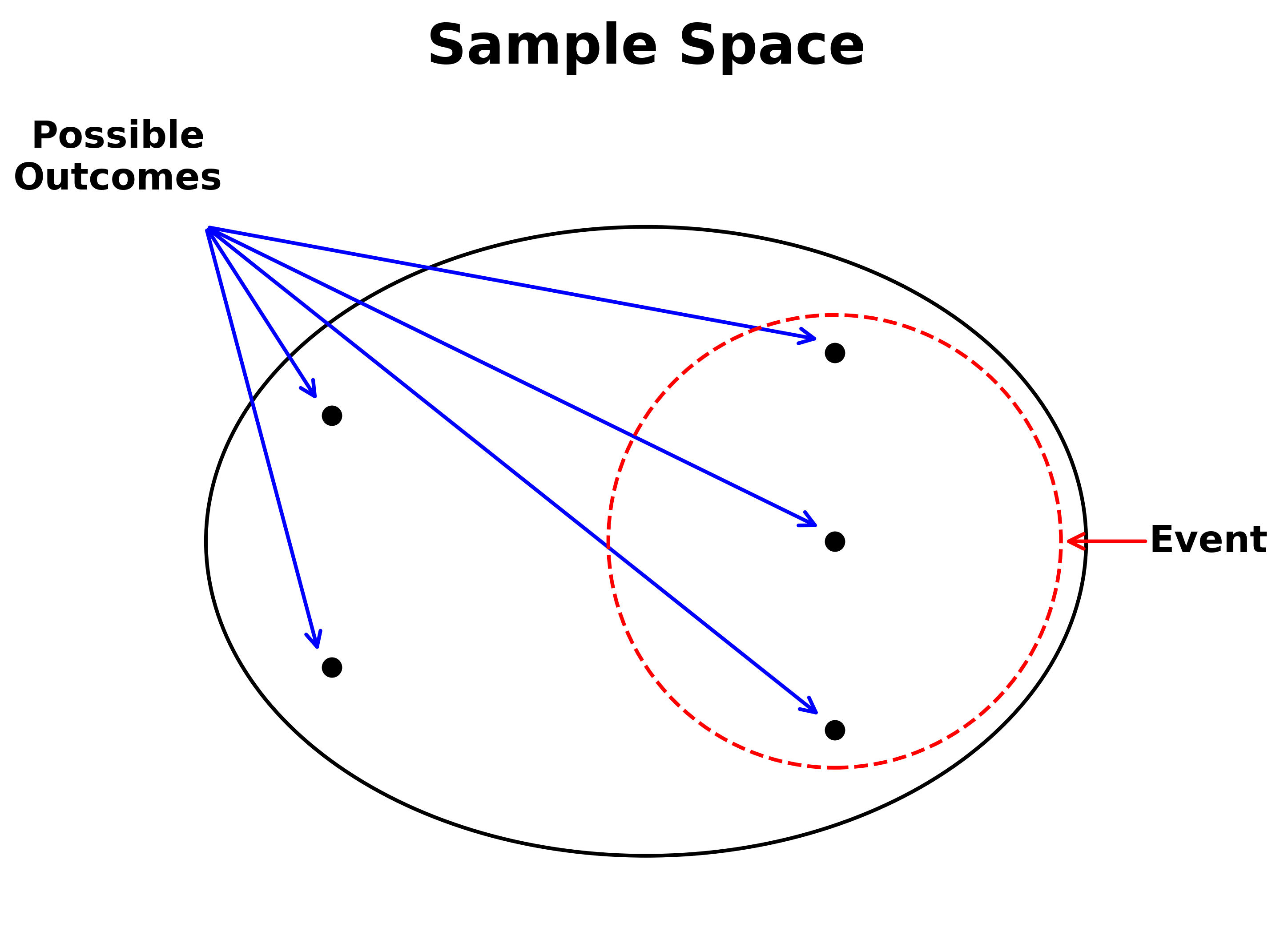
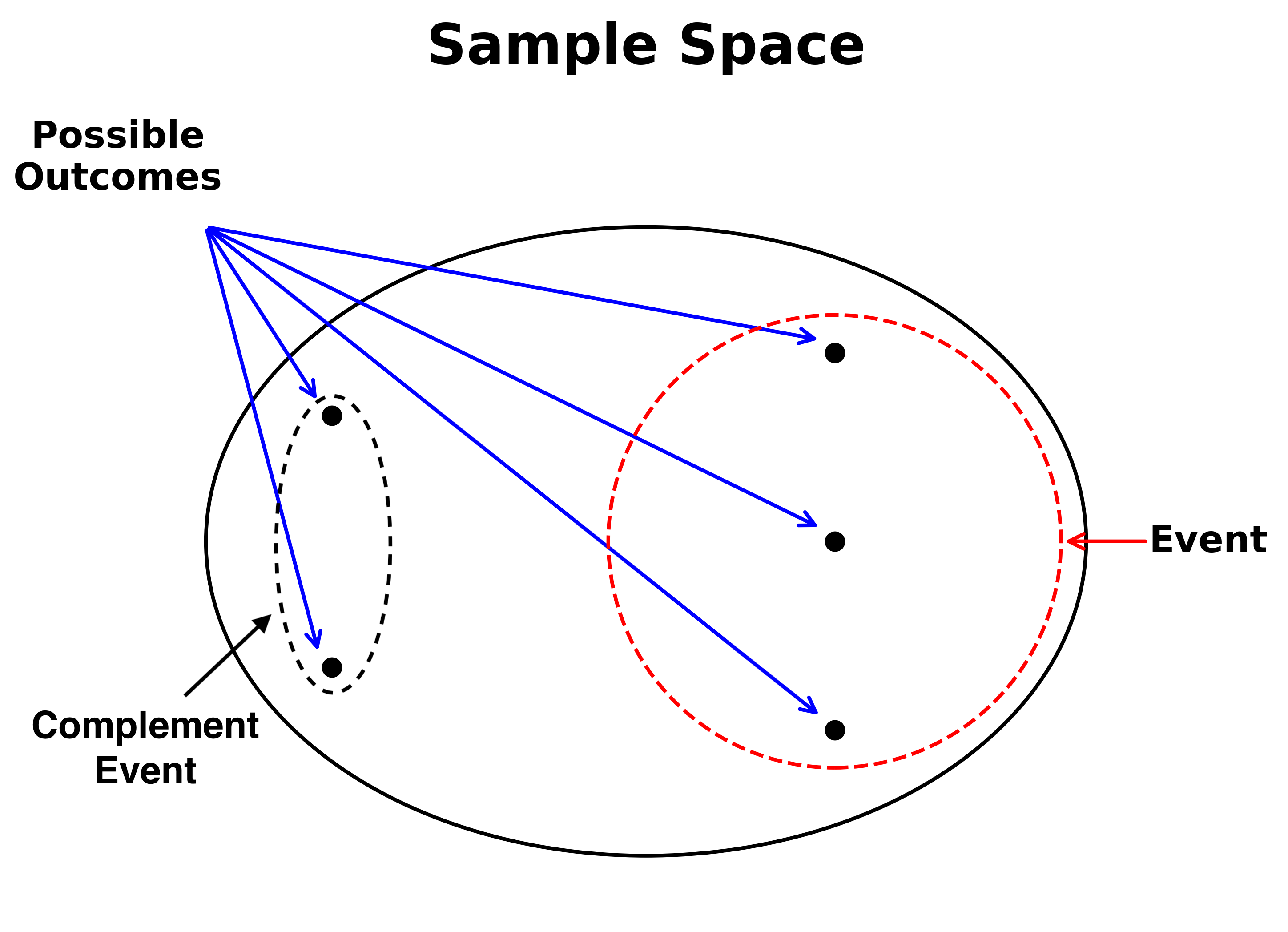
Sample space and outcomes#
The set of possible outcomes is called the sample space.
An event is a collection of some of the possible outcomes.
If all outcomes are equally likely, then the probability of an event is equal to the number of outcomes in the event divided by the total number of possible outcomes.
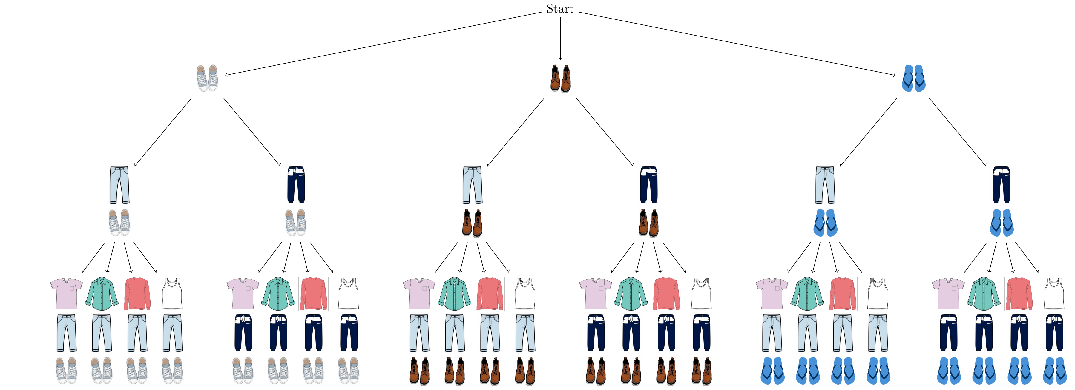
Computing probabilities#
The multiplication rule
Complement rule
Coincidences#
Even if an event is rare, it is likely to happen when there are many opportunities for the rare event to take place.
Examples:
The birthday paradox
Winning streaks
Unit 4: multiple testing!
Conditional probability#
Updating probabilities based on partial information
Bayes’ rule
Common mistakes in conditional probability:
Base rate fallacy: the conditional probability is not informative by itself (librarians vs. farmers)
\(\Pr[A \mid B] \neq \Pr[B \mid A]\) (distracted driving, gateway drugs)
Failing to condition on important information (OJ Simpson)
Generalizing from a biased sample or failing to realize you have conditioned (hot guys are jerks, selection bias)
Unit 4: Estimates, hypothesis testing and experiments#
Statistical significance#
Statistically significant means that the results are unlikely to have occurred by random chance alone.
A p-value is the probability of finding a result at least as extreme/surprising, if outcomes happened by random chance alone.
The null hypothesis corresponds to “just chance” or “no effect.”
The alternative hypothesis corresponds to “better than chance” or “an effect.”
Computing p-value by simulation#
A simulation shows what the results would have looked like if the null hypothesis was true.
Computing the proportion of repetitions that were at least as extreme as the observed data gives the p-value.
Can be one-sided or two-sided.

Experiments#
Drawbacks of observational studies (marshmallow experiment)
Correlation vs. causation and confounding/hidden variables
Effect of selection bias
Potential outcomes model
Computing p-values with simulations and permutation tests
Estimates#
Sample vs. population
Sample size matters for estimation!
The standard deviation of the sample mean is \(\frac{\sigma}{\sqrt{n}}\)
To get \(10\) times more accurate, you need \(100\) times more samples.
Confidence intervals#
For large samples, the distribution of the sample mean is described by the “normal distribution.”
This can be used to make confidence intervals:
\(\hat{\mu}_n \pm \frac{\hat{\sigma}_x}{\sqrt{n}}\) is a 68% confidence interval.
\(\hat{\mu}_n \pm 2 \times \frac{\hat{\sigma}_x}{\sqrt{n}}\) is a 95% confidence interval.
\(\hat{\mu}_n \pm 3 \times \frac{\hat{\sigma}_x}{\sqrt{n}}\) is a 99% confidence interval.
For proportions, \(\hat{\sigma}_x = \sqrt{\hat{\pi}_n(1-\hat{\pi}_n)}\) where \(\hat{\pi}_n\) is the sample proportion.
Unit 5: Machine Learning and Regression#
Predictions#
Statistics is often concerned with making predictions.
On observation \(x\), predict outcome \(y\).
\(x\) is symptoms/test results, \(y\) is diagnosis
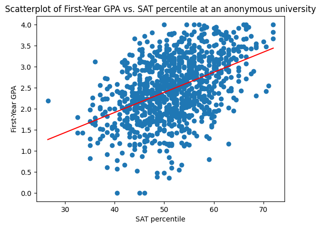
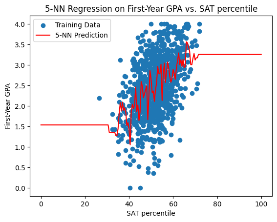
\(x\) is SAT score, \(y\) is first-year GPA
\(x\) is weather now, \(y\) is weather later
We construct a simple model \(f\) so that \(f(x) = \hat{y}\), with the goal that \(\hat{y}\) is as close to \(y\) as possible.
Building models#
It is easier to learn from examples than build a model by hand
Use “training” data to build the model and “testing” data to evaluate the model.
Types of prediction problems
Regression (predicting a quantitative \(y\)).
Classification (predicting a categorical \(y\)).
Text generation (predicting the next word in a sentence).
Examples of models#
Linear and quadratic regression
\(k\)-nearest neighbors
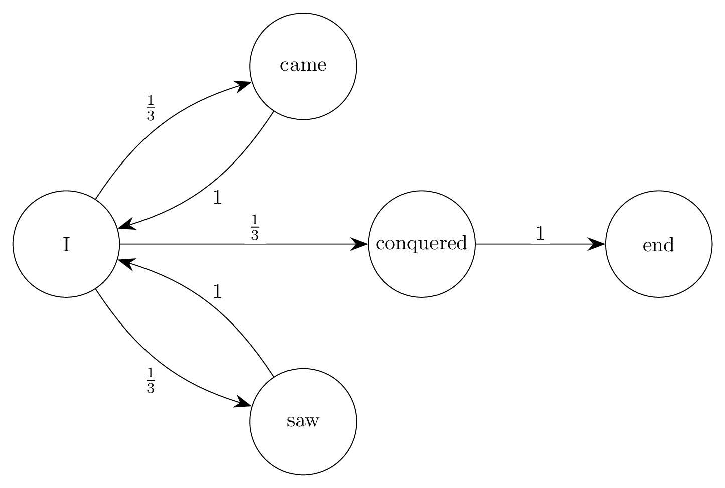
Markov text generators
Training data is everything!#
Selection bias in training data leads to biased models.
If \(x\) is far from all training examples, \(f(x)\) is probably not that accurate for predicting \(y\).
More (good) data and better coverage improves performance.
tl;dr: three themes#
The three major ideas that I want you to take away from this class.
Theme 1: Insight from simple models#
The world is complicated.
Answering a question exactly is overwhelming and often impossible.
Strategy: construct a simple model of the situation.
At least within the simple model, we have the power to answer questions precisely and often quantitatively.
Theme 1: examples#
Ballpark estimates and cost-benefit analysis.
Hypothesis testing.
Machine learning and prediction.
Decision-making in sports
With great power comes great responsibility.
Know the strengths and limitations of your model.
Theme 2: Conditioning matters#
We might understand an uncertain situation well, but everything can change if we condition!
Common mistakes in conditional probability
Selection bias and sampling bias
Hot guys are jerks
Biased estimates and biased ML predictions from biased training data
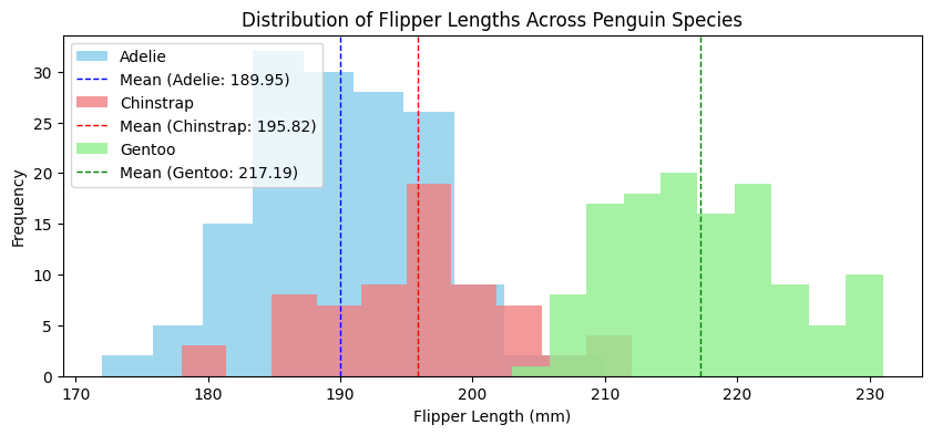
Multi-modal data affects interpretation of summary statistics
Male vs. female penguin body mass
Does generic medical advice apply to you?
Theme 3: Critical thinking is essential#
Once you specify the model, statistics can give precise answers.
Is our model good? Does it fit the situation?
Think critically! Don’t calculate blindly.
Theme 3: examples#
“When means mislead”
Usefulness of fundamental summary statistics (mean, median, standard deviation) depends on data (outliers, skew)
Correlation vs. causation
Confounding variables
Experimental design
Misleading graphs and figures
Multiple testing and \(p\)-hacking
Thinking critically#
We did a lot of “what does this mean in plain English?” exercises.
Thinking like this is important—I do this in my research and in my daily life constantly.
Even though a concept is formal and/or technical, we can and should try to really understand.
Feedback#
I want to make STATS60 great!
Please take a couple of minutes to give some feedback on the course this quarter.
I’m stats-curious. What’s next?#
If you like exploratory data analysis#
DATASCI 112: Principles of Data Science
Deeper dive into data visualization and data analysis
More machine learning: how to train and evaluate ML models
Learn some programming essentials
If you like probability#
STATS 117: Introduction to probability theory
Dive into probability theory
Simple discrete models (coinflips, bags of marbles)
Continuous models (Normal)
STATS 118: Probability theory for statistical inference
Deeper dive into probability theory
The theory behind the normal approximation
Math behind other hypothesis tests
If you like experiments and hypothesis testing#
STATS 191: Introduction to Applied Statistics
Deeper dive into methods for data analysis and prediction
Applications to biology and social sciences
After taking probability theory,
STATS 200: Introduction to Theoretical Statistics
Hypothesis testing
Estimation and confidence intervals
Bayesian methods
Some theory of machine learning
If you like machine learning#
CS 106EA: Exploring artificial intelligence
Training and evaluating ML models
How do neural networks work?
Challenges in ML: over-fitting, bias, distribution shift
After taking MATH 51 and CS 106:
CS 129: Applied Machine Learning
More ML models:
logistic regression
support vector machines
deep learning
“Unsupervised learning”: clustering and feature discovery