The Methodology of Knockoffs - Outline
Why controlled variable selection is hard
A multitude of machine learning tools have been developed for the purpose of predicting a response variable from a vector of covariates, inspiring sophisticated variable selection techniques. To name a few examples, think of penalized regression or non-parametric methods based on trees and ensemble learning. Many of these techniques are extremely popular and enjoy wide applications.
This begs the following question: how do we make sure that we do not select too many null variables? In statistical terms, how do we control for a Type-I error?
For simplicity, consider for a moment the typical example of the lasso:
\[ \begin{align*} \hat{\beta}(\lambda) = \arg\min_{\beta \in \mathbb{R}^p} \left\{ \frac{1}{2} \|Y - X\beta \|_2^2 + \lambda \| \beta \|_1 \right\}. \end{align*} \]
By varying the regularization parameter \(\lambda\) (perhaps tuning it with cross-validation), we obtain different models in which more or less variables have a non-zero coefficient. Intuitively, it seems reasonable to select variables whose fitted coefficient is (in absolute value) above some significance threshold. However, it is not an easy task to choose the threshold (or the value of \(\lambda\)) in such a way as to control the Type-I error.
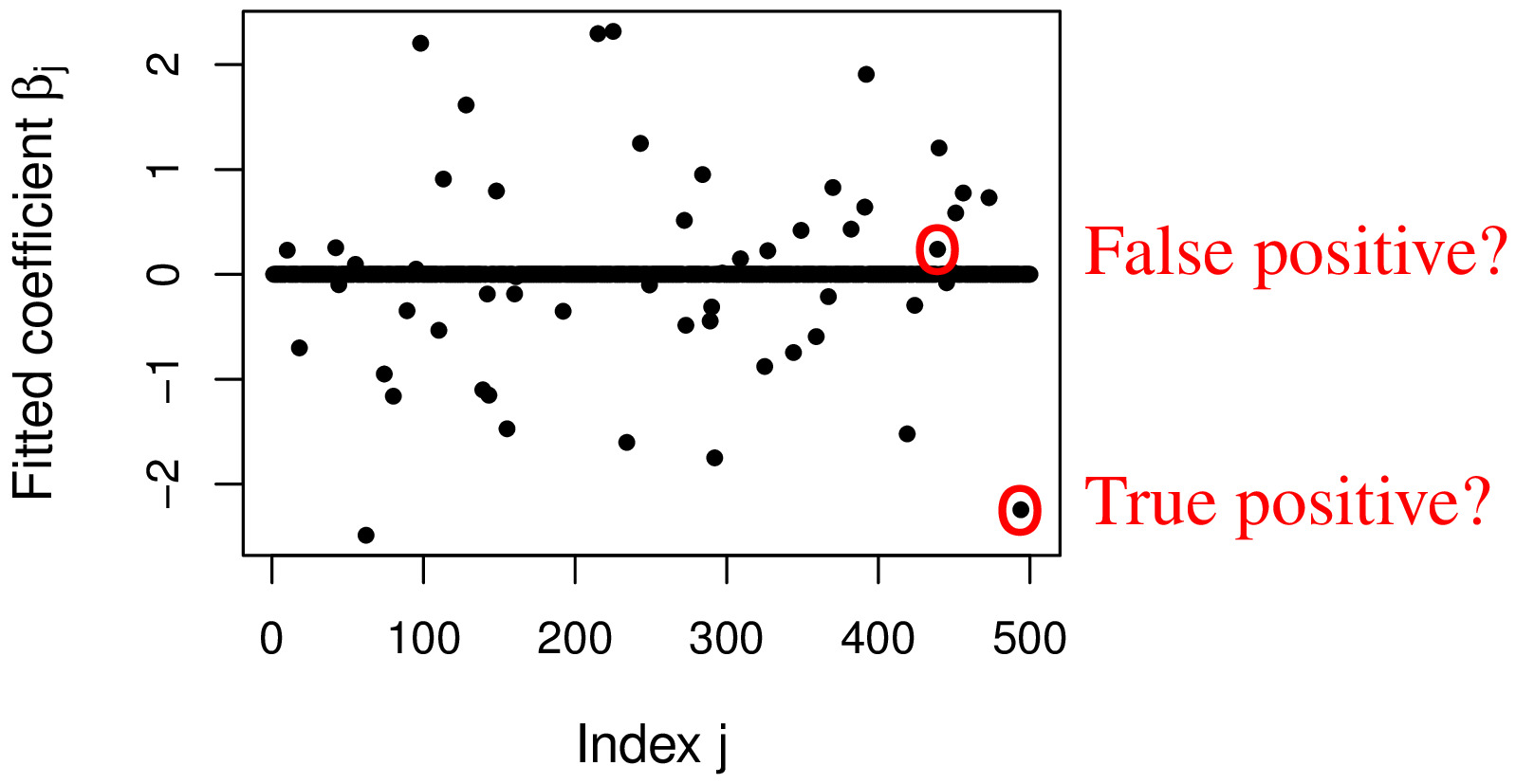
The difficulty arises from the distribution of the estimated coefficients for the null variables being unknown, but at least some of them most likely being non-zero. Moreover, the fitted coefficients are correlated among each other and an incorrect threshold can yield either a very high proportion of false discoveries (if too low) or very low power (if too high).
How knockoffs work
Knockoffs solve the controlled variable selection problem by providing a negative control group for the predictors that behaves in the same way as the original null variables but, unlike them, is known to be null.

The construction of the knockoffs
A rigorous definition of knockoffs depends on some additional modeling choices, but intuitively their nature can be understood as follows.
For each observation of a predictor \(X_j\), we construct a knockoff copy \(\tilde{X}_j\), without using any additional data, such that:
the correlation between distinct knockoffs \(\tilde{X}_j\) and \(\tilde{X}_k\) (for \(j \neq k\)) is the same as the correlation between \(X_j\) and \(X_k\),
the correlation between \(X_j\) and \(\tilde{X}_k\) (for \(j \neq k\)) is the same as the correlation between the original variables \(X_j\) and \(X_k\),
the knockoffs are created without looking at \(Y\).
By construction, the knockoffs are not important for \(Y\), since they are created without even looking at it (as long as the original predictors \(X\) are not removed from the model).
Knockoffs can be used as negative controls for the original variables. The true importance of an explanatory variable \(X_j\) can be deduced by comparing its predictive power for \(Y\) to that of its knockoff copy \(\tilde{X}_j\).
Measuring variable importance
Having constructed the knockoffs, we can proceed by applying a traditional variable selection procedure on the augmented set of predictors \([ X \; \tilde{X} ]\). For each \(j=1,\ldots,p\), we compute statistics \(Z_j\) and \(\tilde{Z}_j\) measuring the importance of \(X_j\) and \(\tilde{X}_j\), respectively, in predicting \(Y\). For instance, we can apply the lasso on the augmented data and compute:
\[ \begin{align*} & Z_j = |\hat{\beta}_{j}(\lambda)|, & \tilde{Z}_j = |\hat{\beta}_{j+p}(\lambda)|, && j=1,\ldots,p. \end{align*} \]
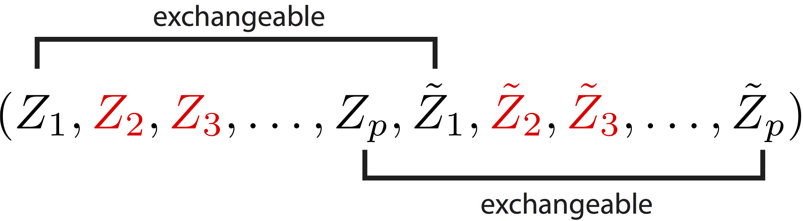
The knockoff filter works by comparing the \(Z_j\)'s to the \(\tilde{Z}_j\)'s and selecting only variables that are clearly better than their knockoff copy. The reason why this can be done is that, by construction of the knockoffs, the null statistics are pairwise exchangeable. This means that swapping the \(Z_j\) and \(\tilde{Z}_j\)'s corresponding to null variables leaves the joint distribution of \((Z_1, \ldots, Z_p, \tilde{Z}_1, \ldots, \tilde{Z}_p)\) unchanged.
Despite the simple example that we presented, the knockoffs procedure is by no means restricted to statistics based on the lasso, as many other options are available for assessing the importance of \(X_{j}\) and \(\tilde{X}_j\). In general, it is required that the method used to compute the \(Z_j\) and \(\tilde{Z}_j\)'s satisfy a fairness requirement, so that swapping \(\tilde{X}_j\) with \(X_j\) would have the only effect of swapping \(Z_j\) with \(\tilde{Z}_j\). However, under certain modeling scenarios, an additional sufficiency requirement is also required.
Once the \(Z_j\) and \(\tilde{Z}_j\)'s have been computed, different contrast functions can be used to compare them. In general, we must choose an anti-symmetric function \(h\) and we compute the symmetrized knockoff statistics
\[ \begin{align*} & W_j = h(Z_j, \tilde{Z}_j) = - h(\tilde{Z}_j, Z_j), && j=1,\ldots,p, \end{align*} \]
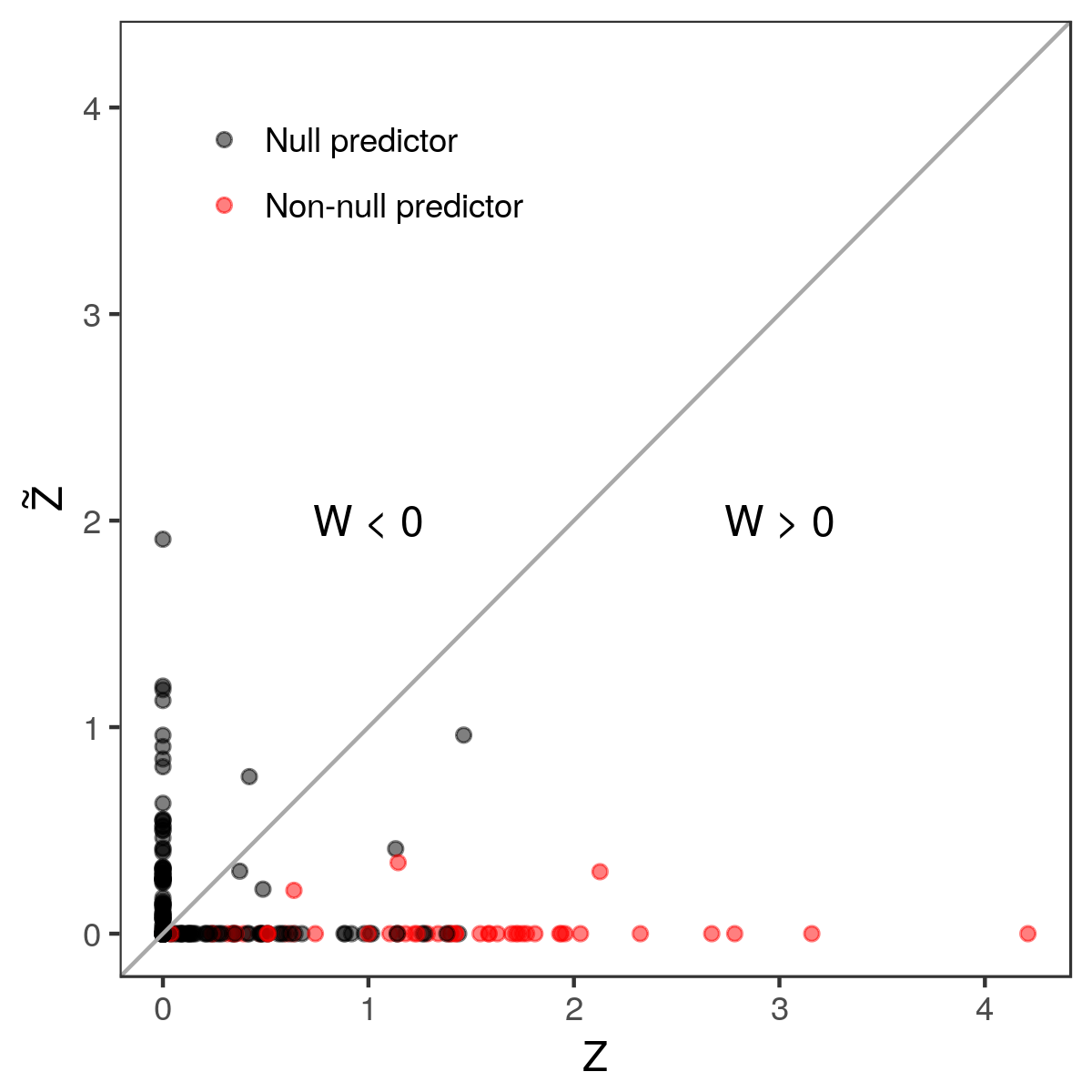
such that \(W_j>0\) indicates that \(X_j\) appears to be more important than its own knockoff copy. A simple example may be \(W_j = Z_j-\tilde{Z}_j\), but many other alternatives are possible.
The figure below shows one realization of the random vector \((Z, \tilde{Z})\), and it seems apparent that the nulls (black dots) are distributed symmetrically around the diagonal. For the non-nulls (red dots) on the other hand, we see a propensity for \(Z_j\) to be larger than its “control value” \(\tilde{Z}_j\) (points below the diagonal).
A data-adaptive significance threshold
Finally, the knockoff procedure selects predictors with large and positive values of \(W_j\), according to the adaptive threshold defined as
\[ \begin{align*} T = \min \left\{ t : \frac{1 + \#\{j : W_j \leq -t \}}{\#\{j : W_j > t \} } \leq \alpha \right\}, \end{align*} \]
where \(\alpha\) is the (desired) target FDR level.
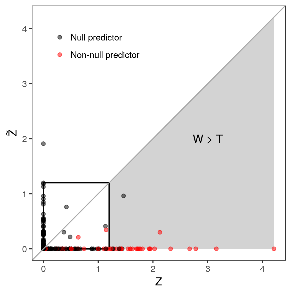
Intuitively, the reason why this procedure can control the FDR is that, by the the exchangeability property of the null \(Z_j\) and \(\tilde{Z}_j\)'s, it can be shown that the signs of the null \(W_j\)'s are independent coin flips, conditional on the absolute values \(|W|\). Consequently, it can be shown that the fraction inside the definition of the adaptive threshold \(T\) is a conservative estimate of proportion of false discoveries.