Esoteric Data Structures: Skip Lists and Bloom Filters
CS 106B: Programming Abstractions
Autumn 2020, Stanford University Computer Science Department
Lecturers: Chris Gregg and Julie Zelenski

Slide 2
Announcements
- Your personal project write-up is due Sunday, 11:59pm
Slide 3
Today's Topics
- Skip Lists
- Bloom Filters
Slide 4
Esoteric Data Structures
- In CS 106B, we have talked about many standard, famous, and commonly used data structures: Vectors, Linked Lists, Trees, Hash Tables, Graphs.
- However, we only scratched the surface of available data structures, and data structure research is alive and well to this day.
- If you want take further classes on data structures, check out Kieth Schwartz's CS 166 Data Structures class.
- Let's take a look at two interesting data structures that have interesting properties and you might not see covered in detail in a standard course: the skip list and the bloom filter.
- Both data structures involve probability, which is something we haven't yet seen in a data structure.
Slide 5
Skip Lists
- Note: much of the material for the Skip List part of this lecture was borrowed from a brilliant lecture by Erik Demaine, at MIT.
- A skip list is a balanced search structure that maintains an ordered, dynamic set for insertion, deletion and search
- What other efficient (log n or better) sorted search structures have we talked about?
- Hash Tables? (nope, not sorted)
- Heaps? (nope, not searchable)
- Sorted Array? (kind of, but insert/delete is O(n))
- Binary Trees? (only if balanced, e.g., AVL or Red/Black)
- A skip list is a simple, randomized search structure that will give us O(log N) in expectation for search, insert, and delete, but also with high probability.
- Invented by William Pugh in 1989 – fairly recent! (Okay, not too recent, but most of the data structures we've looked at have been around since the 1950s/60s)
Slide 6
Improving the Linked List
- Let's see what we can do with a linked list to make it better.
- How long does it take to search a sorted, doubly-linked list for an element?
head→14⇔23⇔34⇔42⇔50⇔59⇔66⇔72⇔79
- log(n)?
- Nope!
- It is O(n) – we must traverse the list!
Slide 7
Improving the Linked List
- How might we help the situation of O(n) searching in a linked list?
head→14⇔23⇔34⇔42⇔50⇔59⇔66⇔72⇔79 - What if we put another link in the middle?
middle ⤸ head→14⇔23⇔34⇔42⇔50⇔59⇔66⇔72⇔79 - This would help a little…we could start searching from the middle, but we would still have to traverse the list.
- O(n) becomes … O(n/2), which is just O(n)
- We didn't really help anything!
- We also had to keep track of the middle.
- Maybe we could just keep adding pointers:
23 50 66 ⤸ ⤸ ⤸ head→14⇔23⇔34⇔42⇔50⇔59⇔66⇔72⇔79 - This would help some more, but still doesn't solve the underlying problem.
- We would have to search the pointers, too, so we're basically back to where we started.
Slide 8
Improving the Linked List
- Let's play a game: the list we've been using was chosen for a very specific reason. Any idea what that reason is? Do you happen to recognize the sequence? (If you're from New York City, you might!)
14⇔23⇔34⇔42⇔50⇔59⇔66⇔72⇔79
- These are subway stops on the NYC 7th Avenue line!
- A somewhat unique feature in the New York City subway system is that it has express lines:
14←--→34⇔42←---------→72 ⇕ ⇕ ⇕ ⇕ 14⇔23⇔34⇔42⇔50⇔59⇔66⇔72⇔79 - To search the list (or ride the subway): Walk right in the top list and when youi've gone too far, go back and then down to the bottom list.
- To search for 59 above, start at the 14 in the top list, and then traverse to the 34, then the 42, then the 72. Recognize that you've gone too far, and go back to the 42 and down to the corresponding 42 in the bottom list. Then go to the 50 and then finally to the 59 in the bottom list.
Slide 9
Skip Lists
  L1: 14←--→34⇔42←---------→72
      ⇕     ⇕  ⇕            ⇕
  L2: 14⇔23⇔34⇔42⇔50⇔59⇔66⇔72⇔79
- For the two lists, L1 and L2 above, what is the best placement for the nodes in L1? For the subway, it is based on ridership, but for we want to minimize the worst-case performance.
- We want equally spaced nodes.
- The search cost can be represented as follows:
|L1| + (|L2| / |L1|) - where
|L1|is the number of nodes in L1, and|L2|is the number of nodes in L2. - We always want all the nodes,
n, in L2, so we can represent the search cost as follows:|L1| + (n / |L1|) - We can do a bit of calculus to minimize
|L1|, by taking the derivative with respect to|L1|and setting this equal to 0 (welcome to Calc I!)d(|L1| + (n / |L1|))/d(|L1|) = 1 - n * |L1|^(-2) - We can set this equal to 0 and solve for
|L1|:1 - n * |L1|^(-2) = 0 1 = n / |L1|^2 |L1|^2 = n |L1| = sqrt(n) - So, for two lists, minimizing the number of nodes in the second list would be placing them every
sqrt(n)away from each other. - How does this change our search time in terms of Big O?
- We can plug in
sqrt(n)in for|L1|in our original function, and solve:sqrt(n) + n / sqrt(n) = 2 * sqrt(n) - So, we have O(2 * sqrt(n)) = O(sqrt(n)). Not bad!
- But, not as good as O(log n).
- We can plug in
Slide 10
Skip Lists
- What if we had more lists?
- The search calculations get a bit tricky, but this is the end result:
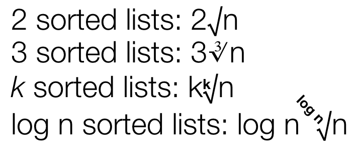
- It turns out that if we have
log nnumber of lists, we have an interesting situation, becuase n^(1 / log2 n) is just equal to 2, which means that we end up with O(2 log2 n), or just O(log n). - This is what we want!
Slide 11
Skip Lists
- What we want to build is the following:
- log n number of lists, with the lowest list with n nodes, the next higher list with n/2 nodes, the next higher list with n/4 nodes, etc., until the top list has a signle node (well, really a node on the left and on the right):
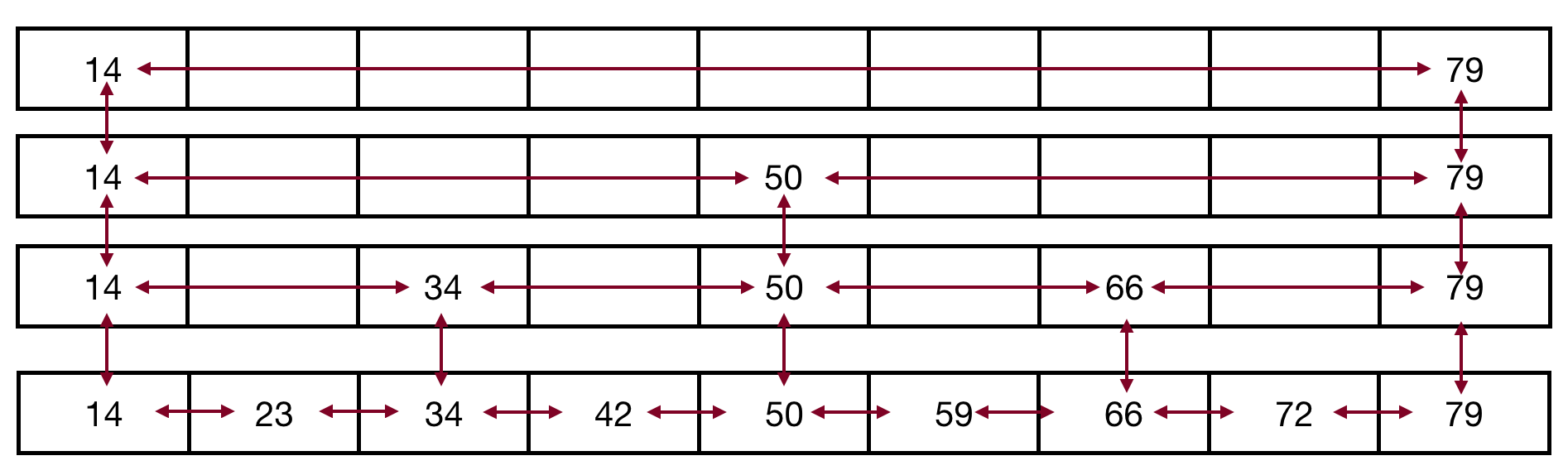
- log n number of lists, with the lowest list with n nodes, the next higher list with n/2 nodes, the next higher list with n/4 nodes, etc., until the top list has a signle node (well, really a node on the left and on the right):
- This should look a bit like a binary search tree, and it acts like one!
Slide 12
Building a Skip List
- The question now is, how do we build a skip list?
- We could try to keep all the elements perfectly aligned – in the lowest list, we have n elements, and in the next list up we have n/2 elements, etc.
- This would not be efficient, becuase we would be moving links all over the place!
- What we do instead is to build the list using a probabilistic strategy
- We flip a coin!
- Here's the algorithm:
- All lists will have a -∞ node at the beginning of the list, in order to make a standard "minimum" node.
- All elements must go into the bottom list (search to find the spot)
- After inserting into the bottom list, flip a fair, two sided coin. If the coin comes up heads, add the element to the next list up, and flip again, repeating step 2.
- If the coin comes up tails, stop.
- Let's build one!
Slide 13
Bloom Filters
- Our second esoteric data structure is called a bloom filter, named for its creator, Burton Howard Bloom, who invented the data structure in 1970.
- A bloom filter is a space efficient, probabilistic data structure that is used to tell whether a member is in a set.
- Bloom filters are a bit odd because they can definitely tell you whether an element is not in the set, but can only say whether the element is possibly in the set.
- In other words: false positives are possible, but false negatives are not.
- (A false positive would say that the element is in the set when it isn’t, and a false negative would say that the element is not in the set when it is).
Slide 14
Bloom Filters
- The idea behind a Bloom Filter is that we have a bit array. We will model a bit array with a regular array, but you can compress a bit array by up to 32x because there are 8 bits in a byte, and there are 4 bytes to a 32-bit number (thus, 32x!) (although Bloom Filters themselves need more space per element than 1 bit).
- This is a bit array:
| 1 | 0 | 1 | 1 | 0 | 1 | 1 | 1 |
- For a bloom filter, we start with an empty bit array (all zeros, indexes added), and we have
khash functions:k1 = (13 - (x % 13)) % 8 k2 = (3 + 5x) % 8 etc.
| 0 | 1 | 2 | 3 | 4 | 5 | 6 | 7 |
| 0 | 0 | 0 | 0 | 0 | 0 | 0 | 0 |
- The hash functions should be independent, and the optimal amount is calculable based on the number of items you are hashing, and the length of your table (see the Wikipedia article on Bloom Filters for details).
- To insert a value, hash the value with all
khashes, and then set the bit in the hashed position to 1 for each result.
Slide 15
Bloom Filter Example Insertions
- Insert 119:
x = 119k1 = (13 - (x % 13)) % 8 = 3k2 = (3 + 5 * x) % 8 = 6
- Because
k1is 3, we change bit 3 to1. Becausek2is 6, we change bit 6 to1:
| 0 | 1 | 2 | 3 | 4 | 5 | 6 | 7 |
| 0 | 0 | 0 | 1 | 0 | 0 | 1 | 0 |
- Insert 132:
x = 132k1 = (13 - (x % 13)) % 8 = 3k2 = (3 + 5 * x) % 8 = 7
- Because
k1is 3, we don't change the array, because bit 3 is already a1. Becausek2is 7, we change bit 7 to1:
| 0 | 1 | 2 | 3 | 4 | 5 | 6 | 7 |
| 0 | 0 | 0 | 1 | 0 | 0 | 1 | 1 |
Slide 16
Bloom Filters: Determining if a value is in the set
- To check if values are in the set, re-hash with all the hash functions. If the bits returned are
1, then we can say that the value is probably in the table.- Why probably? There is overlap, and we could potentially have two values overlap bits such that another value will appear as if it was inserted.
- Example from above:
- To see if 119 is in the set, we re-hash:
k1 = 3,k2 = 6: - 119 is probably in the set (and we did add it to the set)
- To see if 119 is in the set, we re-hash:
- Another example: search for 126 in the set:
k1 = 4,k2 = 1- 126 is definitely not in the set. Why?
- There are 0s in the resulting bits (both index 4 and index 1 have 0s)
- Another example: search for 143:
k1 = 5,k2 = 6- 143 is definitely not in the set. Why?
- There are 0s in the resulting bits (index 5 is 0)
- Another example: search for 175:
k1 = 7,k2 = 6:- 175 is probably in the set. Why?
- Both bits 6 and 7 are
1. - But, we never entered 175 into the set! This is a false positive, and we can't rely on positive values.
- Here is a great online example to see how Bloom Filters work: https://llimllib.github.io/bloomfilter-tutorial/
Slide 17
Bloom Filters: Probability of a False Positive
- What is the probability that we have a false positive? Let's do a bit of math.
- If \(m\) is the number of bits in our bit array, then the probability that a bit is not set to
1is:
- If \(k\) is the number of hash functions, the probability that the bit is not set to
1by any hash function is:
- If we have inserted \(n\) elements, the probability that a certain bit is still
0is:
- To get the probability that a bit is
1is just1 -the answer previous calculation:
- Now we test membership of an element that is not in the set. Each of the \(k\) array positions computed by the hash functions is
1with a probability as above. The probability of all of them being1, (false positive) is:
- For our prior example, \(m = 8\), \(n = 2\), and \(k = 2\), so:
- or 17% of the time we will get a false positive.
Slide 18
Bloom Filters: Why?
- Why would we want a structure that can produce false positives?
- Example: Google Chrome uses a local Bloom Filter to check for malicious URLs — if there is a hit, a stronger check is performed.
- There is one more negative issue with a Bloom Filter: you can’t delete! If you delete, you might delete another inserted value, as well! You could keep a second bloom filter of removals, but then you could get false positives in that filter…
- One other thing: Big O?
- You have to perform k hashing functions for an element, and then either flip bits, or read bits. Therefore, they perform in O(k) time, which is independent of the number of elements in the structure. Additionally, because the hashes are independent, they can be parallelized, which gives drastically better performance with multiple processors.