Lab 2: Capturing Airband Signals with MATLAB and your RTL-SDR
Overview
Last week you used an integrated program, gqrx or SDR#, to control your SDR and listen to commercial FM, along with a range of other frequencies. This week we'll get a little closer to the hardware, and learn how to control the SDR's more directly. We'll use MATLAB's support for the rtl-sdr to read data directly, so that we can examine and decode it. We'll capture AM signals in the airband.
Aims of the Lab
This week we'll look at other ways to control your SDR to capture AM airband data with MATLAB and process it. You will capture a signal, display it's spectrum as an image, decode the signal, plot it, and play back the audio.
MATLAB Hardware Support for the RTL-SDR
First we will need to load some packages into MATLAB. This includes hardware support for the rtl-sdr, as well as the communications and signal processing toolboxs. You can add these from within MATLAB by clicking on the "Add-ons" button. This brings us to a pulldown menu
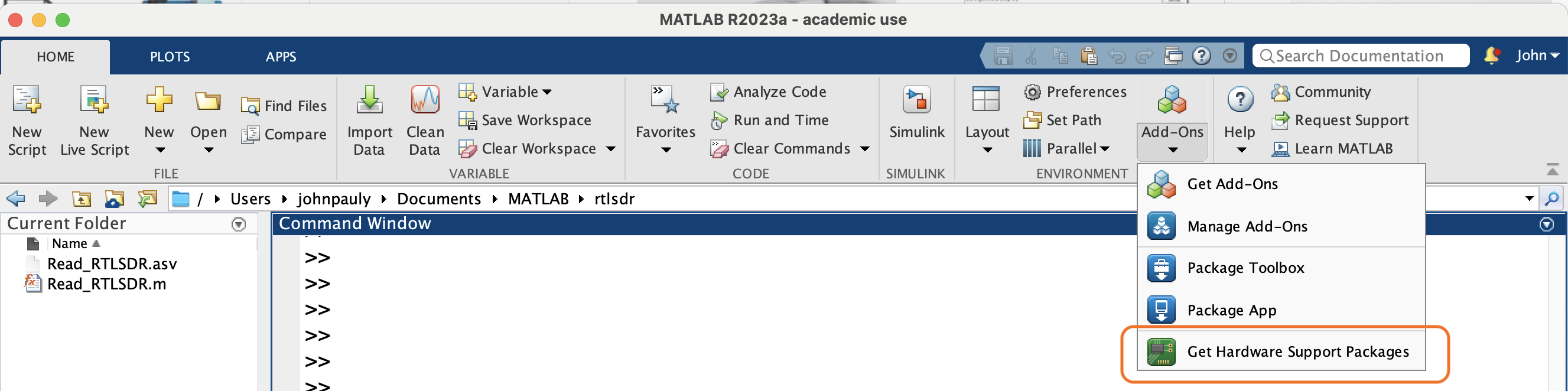
Click the "Get Hardware Package Support" entry. This brings up a page for all of the different types of hardware MATLAB knows how to work with, including several sdr's, including the rtl-sdr that we are using. The page looks like

Click on the rtl-sdr enrty, here in the lower right of the page. This brings up a page for installing the packages you need.
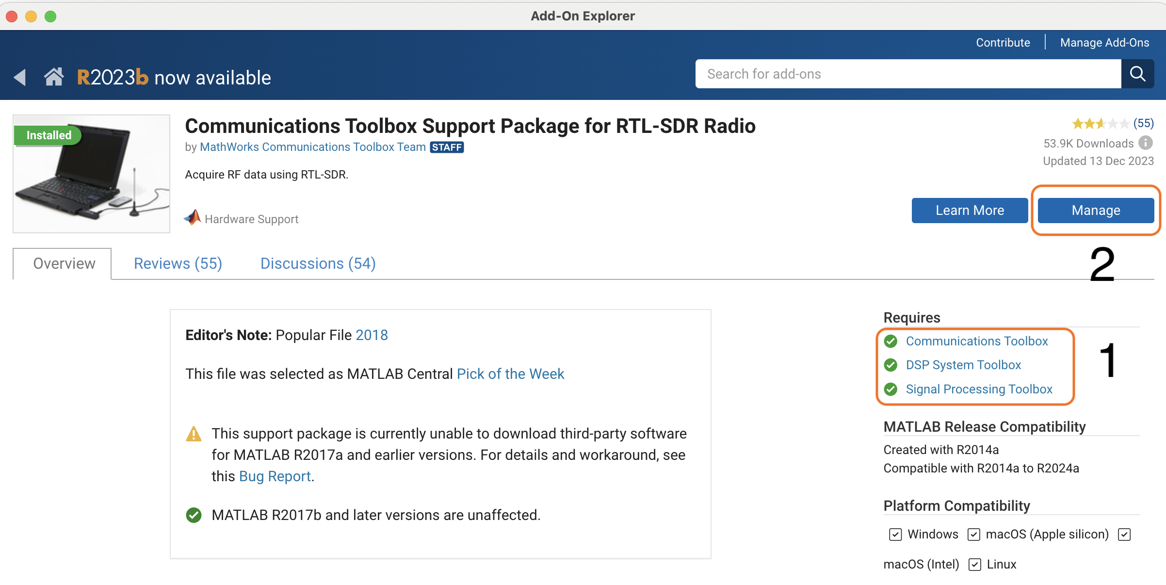
First check that you have the requirements, in the box labeled 1. These are links to other installation pages. You probably have all these already. Then click the second button to install the rtl-sdr drivers and routines. Mine says "Manage" because I've already installed everything. Yours will say "Install". Follow the instructions on that page, including plugging your sdr in, and running the initialization process from the pop up window. At this point you should be all set. If you are a windows user, you already have the driver installed, so you can skip that step.
The documentation for the MATLAB package can be found with
You can check to see if your setup is working by first plugging the rtl-sdr in, and then running
>> sdrinfo

ans =

                RadioName: 'Generic RTL2832U OEM'
             RadioAddress: '0'
              RadioIsOpen: 0
                TunerName: 'R820T'
             Manufacturer: 'Realtek'
                  Product: 'RTL2838UHIDIR'
               GainValues: [29×1 double]
      RTLCrystalFrequency: 28800000
    TunerCrystalFrequency: 28800000
             SamplingMode: 'Quadrature'
             OffsetTuning: 'Disabled'
Acquiring RF Data from MATLAB
MATLAB has a number of different ways to interact with the rtl-sdr. For now we are just going to use it to collect a frame of several seconds of RF data, which we can then process using MATLAB's signal processing tools, and then play back the result.
The routine to do this is
function y = Read_RTLSDR(cf, sf, fs, nf ,g)
%
% Utility to read data from an rtl-sdr
%
% y = Read_RTLSDR(cf, sf, fs, nf, g)
%
% Inputs:
%   cf - center frequeny in Hz (88.5e6 for KQED)
%   sf - sampling frequecy in Hz, typically 2.048e6
%   fs - frame size, typically 1e5
%   nf - number of frames
%   g  - reciever gain in dB, typically 10 to 30
%
% Returns:
%   y - complex I and Q samples of the RF waveform
%
% The total acquisition time is (fs*nf)/sf seconds
%
% Choose the gain so that the amplitude is less than 128, where
%    the rtl-sdr clips, but large enough you can't see the quantization
%

% set up the rtl-sdr
hSDR = comm.SDRRTLReceiver('0', ...
              'CenterFrequency',  cf, ...
              'SampleRate',       sf, ...
              'SamplesPerFrame',  fs, ...
              'EnableTunerAGC',false);
% we can't do this in the call above for some reason!
hSDR.TunerGain = g;

% collect the data
buf = [];
for counter = 1:nf
    buf = [buf; step(hSDR)];
end

% free up the device
release(hSDR);

% convert the data into doubles for MATLAB
y = double(buf);

end
which is available here:
The rtl-sdr is freed after it is used, so that you can run gqrx or sdrsharp. However, you need to quit these before you run the m-file again, or MATLAB hangs, since it can't get access to the device.
Airband AM Signals
The main part of the lab is to capture and decode AM signals in the air band, with is right above the commercial FM band we were decoding last week. There is a band from 108-118 MHz that mostly has navigation beacons that identify themselves by Morse code. Then from 118-137 MHz there are several bands used for communication between aircraft and the ground. Communications in these bands uses AM modulation. This is because when two users try to talk on the same channel, you hear both of them with AM. With FM, you hear only the stronger of the two, or something completely intelligible if both are the same strength. With air traffic control, it is important to hear everyone that is out there!
The local airport is Palo Alto, which is station KPAO. It transmits on these frequencies
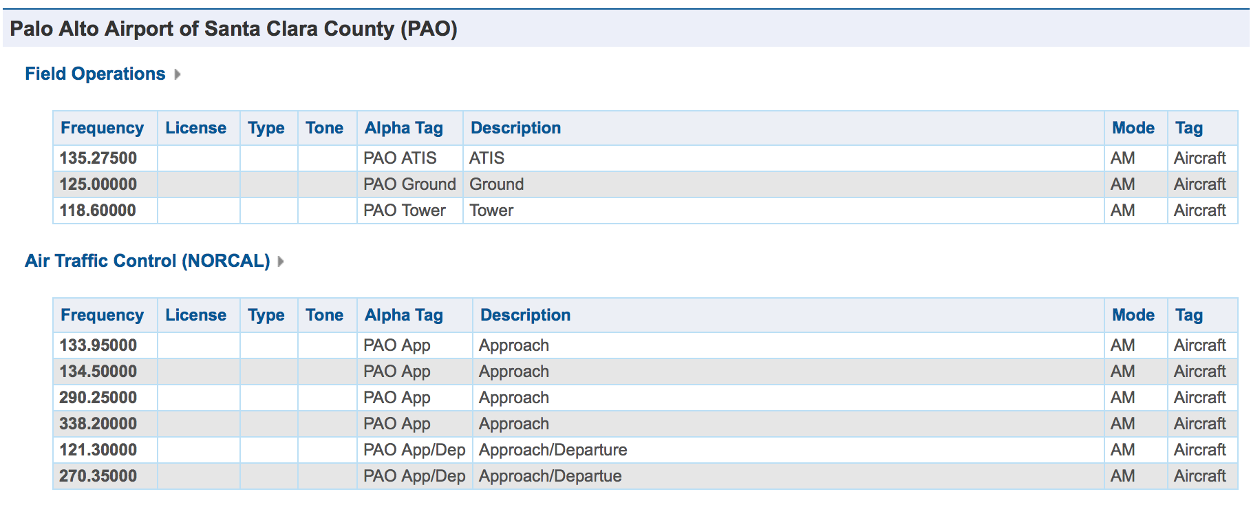
We will also hear traffic from San Francisco (SFO), San Jose (SJC), as well as NORCAL Approach, which coordinates the airspace. The frequencies for SFO are
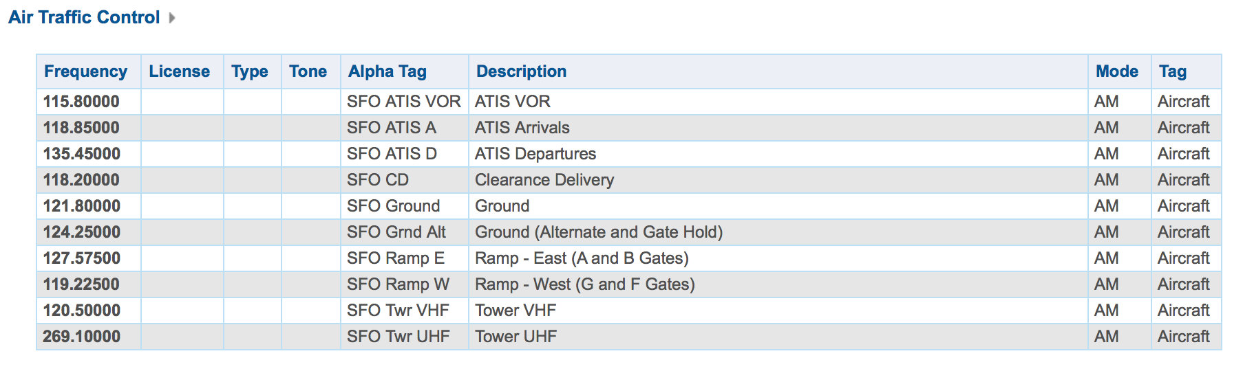
and San Jose are
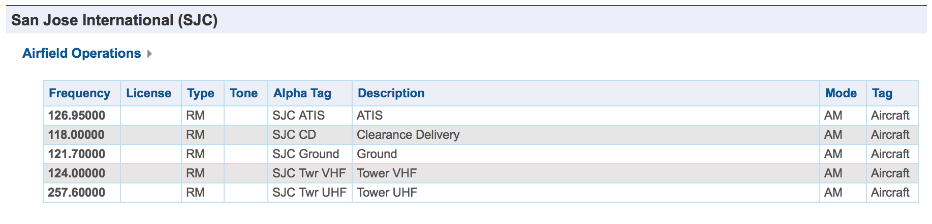
and Norcal Approach are
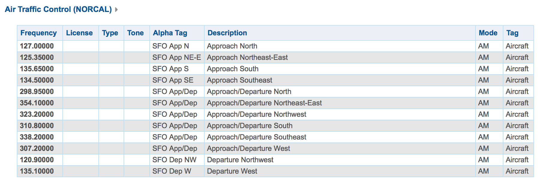
Choose a frequency where you might expect to get a signal. The ATIS frequencies are good initial candidates, because these continuously transmit information about the airport, and how to contact them. The other frequencies, such at the air traffic control frequencies, are more interesting, but are not always in use. Often a transmission lasts just a few seconds, and can be hard to capture.
One busy channel that has a strong signal around here is 310.8 MHz, SFO departures and arrivals from the south. This frequency also is a good match for your SDR antenna. At 310.8 MHz a quarter wave antenna is 24 cm, or about 9.5 inches. Stick your antenna to a metal surface to provide a ground plane, and extend the antenna to this length. Small adjustments to the frequency can help (+/- a few kHz).
Use gqrx or SDR# to see if you can find any activity. Here is an example
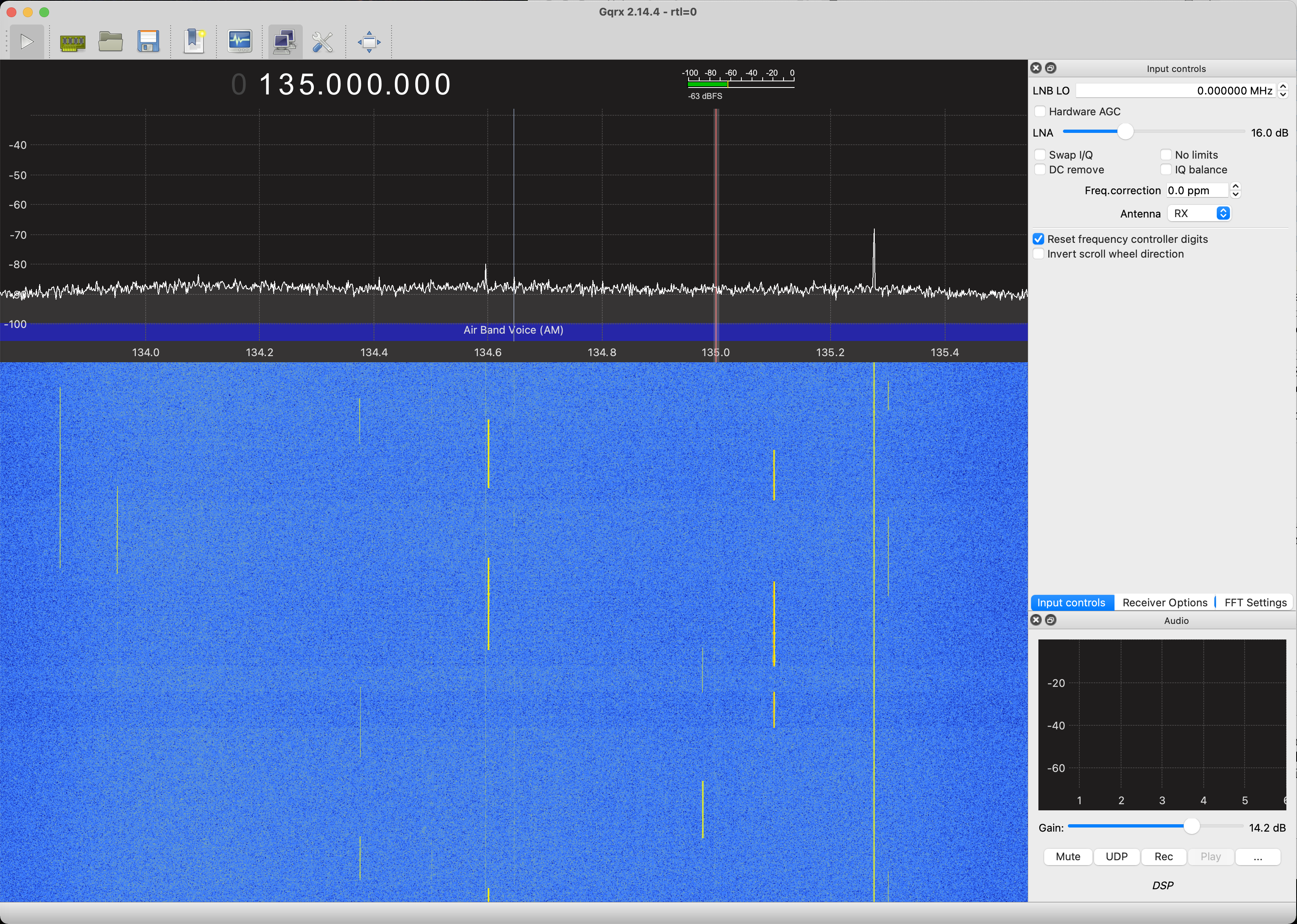
You see a couple of frequencies in use. The one that is on continuously is an ATIS signal. The others are planes and towers talking to each other. Note the gain you use here, so you can set it to be the same for your capture.
Once you know there is a signal out there, capture 8 seconds of data, and save it to a file. Close gqrx or SDR# to free up the SDR, and then capture the data with
where I have chosen 310.8 MHz, which is Norcal Approach/Departure South. We are setting the frequency exactly to the channel we are interested in to make the processing easier. This is generally a bad idea, as we will see shortly. The data file is available at
You can use this file if you are having trouble finding signals to capture. Another signal you can usually see is the Palo Alto ATIS, since it is close, and transmits all of the time.
The first thing to note is that just 8 seconds of RF is a lot of data! It is hard to tell if we have anything, or how to extract it. What we will do is make something like the waterfall plot that you see in gqrx or SDR#, called a spectrogram. What this does is compute the spectrum of blocks of the signal, and displays an image of how this changes over time. A basic spectrogram program is provided here
It is msg.m for "my spectrogram". We will improve this as the course goes on. The help information is
>> help msg

  msg(x,n0,nf,nt,dbf)

   Computes and displays a spectrogram

       x  -- input signal
       n0 -- first sample
       nf -- block size for transform
       nt -- number of time steps (blocks)
       dbf -- dynamic range in dB (default 40)

   This extracts a segment of x starting at n0, of length nf*nt
   The image plot is in dB, and autoscaled.  This can look very noisy
   if there aren't any interesting signals present.
This takes an input signal starting at sample n0, and computes the spectrum of nt segments of the signal, each of length nf. The result is displayed as an image, with time going horizontally, and frequency vertically. The center frequency is in the middle of the plot. To look at the spectrum for the entire 8 s signal
Unless you have a very big display, you'll get an error message that the image doesn't fit, and was scaled down. The result looks like this
This is 8 seconds of data. The horizontal axis is time, 0 to 8 seconds, and the vertical axis is frequency, -1.2 MHz to 1.2 MHz. The signal we want is right in the middle at 0 MHz. The signal starts at about 2 seconds, and continues to about 7 seconds. Depending on your luck, you may see several signals at other different frequencies.
For now we'll just focus on the signal at 0 MHz. The audio signal has a bandwidth of about +/- 5 kHz, so we need to reduce the sampling rate from 2.4 MHz to 10 kHz. This is called decimation, in this case by a ratio of 2.4e6/10e3 = 240. A lowpass filter first limits the bandwidth to +/- 5 kHz, and then takes every 240th sample.
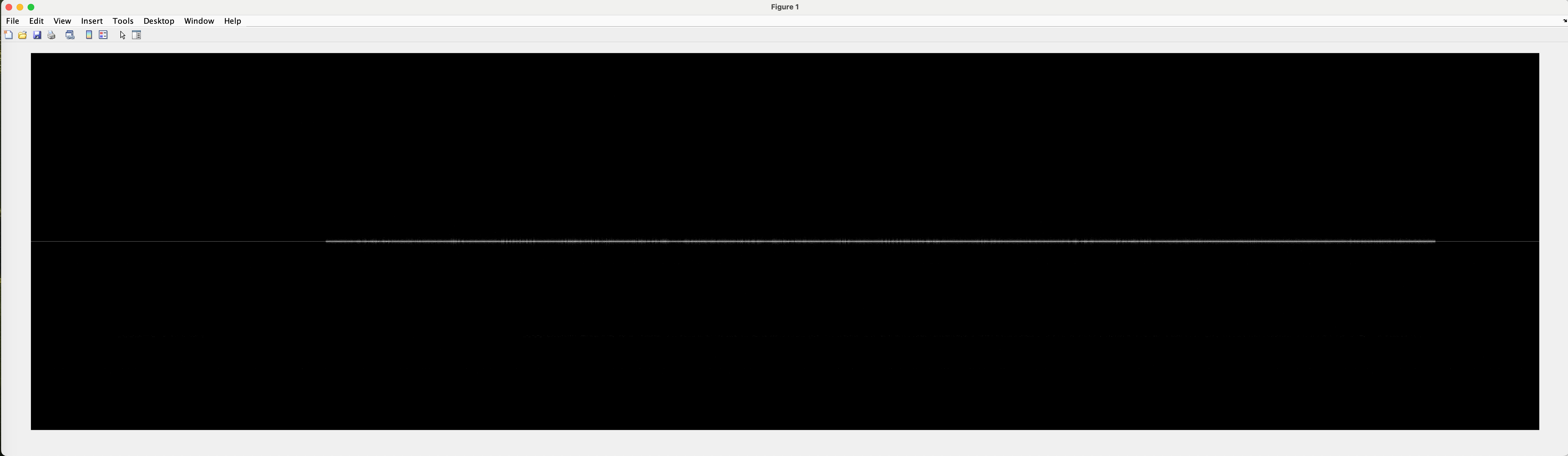
If we plot the magnitude of the decimated signal with
>> t = [1:length(ab310d)]/(2.4e6/240);
>> plot(t,abs(ab310d));
>> xlabel('Time, seconds')
>> ylabel('Magnitude')
we see
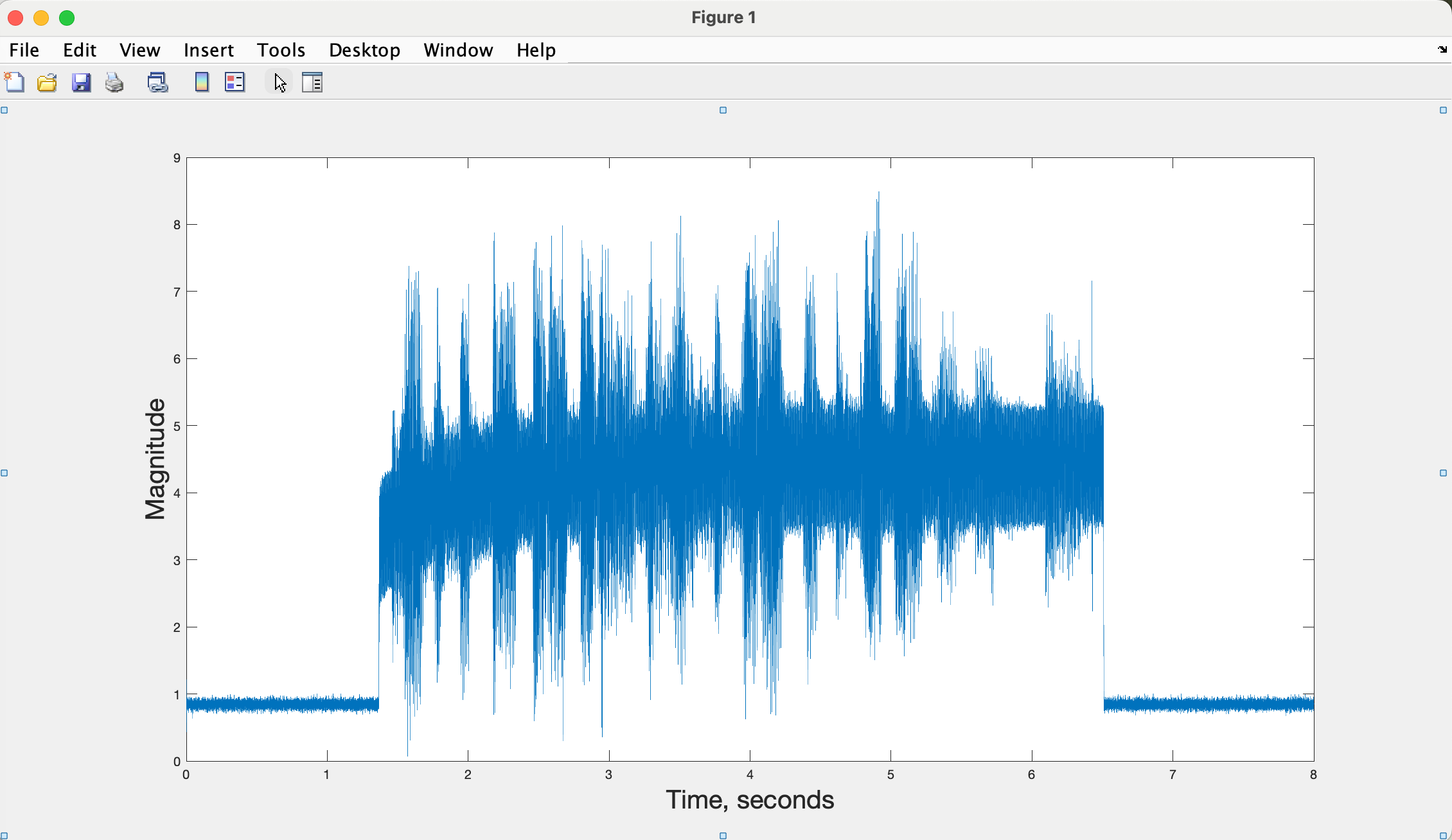
This is a classic AM signal. There is an offset of about 1 unit from the DC feedthrough because we are receiving right at zero frequency. We'll look at fixing this below. Then the AM signal starts at about 1.5 seconds. What you see is the AM offset that biases the audio waveform to make it always positive. On top of that you see the actual audio signal.
You can play the signal with
The factor of 9 scales the waveform to be less than one, which is what sound() requires to avoid clipping, and 10e3 is the sampling rate after decimation. We haven't suppressed the AM offset, because your audio system can't reproduce it anyway.
Your Report
In general you don't want to acquire a signal exactly on frequency. Receivers always have a noise spike there. Acquire another data set where the receive frequency is offset from the signal you are interested in. For the example above, set the receive frequency to 310.7e6, so that you are 100 kHz below the signal you are capturing. A sample data set is here:
Another data set is here:
This is acquired at 135 MHz, just 275 kHz below the Palo Alto ATIS frequency, which is in the data set. It also has a signal from an aircraft that you can find and decode. You can use this data set if you'd like, or the one above, or one you capture yourself.
Since we are not directly on the signal's frequency we need to shift the frequency before we decimate. If d is our raw data vector and fs is the sampling frequency, we can do this with
where f_offset is the frequency you want to shift to. The signal dm should have our signal at the center of the spectrogram.
For your report 1. What happens if we don't shift the frequency and just decimate, as we did above. Plot the signal you get. 1. See if you can center the signal you are interested in, and show the spectrogram in your report. 1. Plot the magnitude of the decimated signal, and include that in your report. Is the DC offset gone? 1. Play back the audio, and describe what you hear. 1. What happens if you decimate by 120, instead of 240? When you play the signal the sampling frequency is now 20 kHz. Describe the difference in the audio quality.
For all of these use screen captures in your report. There is a lot of data, and pdf's can get huge.