Lab 3: Finding Signal in Time and Frequency
Overview
Last week we picked an air traffic control frequency we expected to be in use, and then captured as segment of it with our rtl-sdr's. Thats fine if we know which signal we are looking for. But it wuld be nicer to be able to capture a large band of frequencies, and then find all of the signals later, and play them back. That is what we will do this week. In the end, you could make an air band scanner if you would like.
Aims of the Lab
The objective of the lab is to gain familiarity with where signals are in time, and in frequency. Last week we plotted a spectrogram (or waterfall plot) to depict the entire spectrum. This week we will look at how to find exactly when they start and stop, and exactly what frequency the are.
Air Band Data Sets
First we'll need data to work with. You can capture your own with
>>  % center Frequency, air band
>>  fc = 134.8e6;
>>  % Sampling Frequency
>>  fs = 2.4e6;
>>  % frame size
>>  fr = 240e3;
>>  % Number of frames
>>  nf = 200;
>>  % Gain
>>  g = 30;
>>  d = Read_RTLSDR(fc,fs,fr,nf,g);
This is centered at 134.8 MHz, which is right in the middle of the air band. I chose this so that it captured as many signals as possible. The sampling rate is 2.4 MHz. The frame size (the length of each block o data from the rtl-sdr) is 240e3 samples, which is then 0.1 seconds each. We are capturing 200 frames, for a total of 20 seconds. The Gain here is 30 dB, which is just to the point were very strong signals clip.
Here a a couple of data sets that you can use.
These have up to five different channels active at the same time, each at their own frequency.
Listening to the Whole Band at Once
One surprising trick with AM is that we can easliy listen to everything in the band at once. Since AM encodes the signal in the envelope, we can just compute the magnitude of the entire RF signal, decimate that down to baseband, and play that back.
If we want to reduce the bandwidth from the sampling frequency of 2.4 MHz to 10 kHz, we need to decimate by a factor of 240. Using the first data set,
>>  load ab134.8_d1
>>  d1d = decimate(abs(d1),240);
>>  % Audio frequncy sampling rate
>>  fa = fs/240;
We can plot this with
>>  % Time in seconds
>>  t = [1:length(d1d)]/fa;
>>  plot(t,d1d);
>>  xlabel('Time, s');
>>  ylabel('Magnitude');
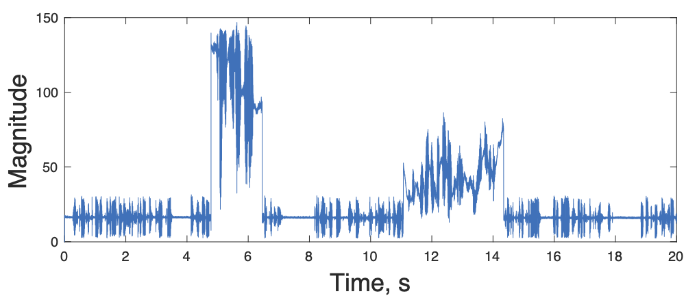
We can also play it back to see what it sounds like
We used soundsc() here because it autoscales the signal, so we don't have to worry about clipping.
There is lots of stuff happening! The Palo Alto Airport ATIS signal is always there as you both see and hear. Stronger signals from aircraft come in every once in a while. If the aircraft signal isn't too strong (the second one), you hear both. If one is much stronger (the first one), we just hear that one. This is one of the reason AM is used for air traffic control. With narrow band FM, as we'll cover in the next lab, all we would get is a buzz with the two interfering signals, and we couldn't understand either of them.
Sometimes there can be much more activity on.
>>  load ab134.8_d2
>>  d2d = decimate(abs(d2),240);
>>  plot(t,d2d);
>>  xlabel('Time, s');
>>  ylabel('Magnitude');
>>  soundsc(d2d, fa);
Looking at the plot you see much more activity and interference:
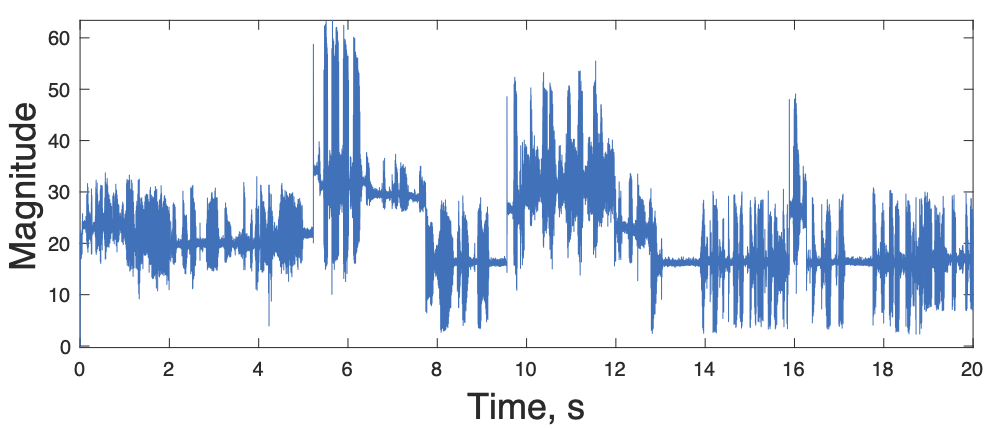
All of the signals are of fairly similar amplitudes, so they all interfere. How do we sort them out?
Last time we used a spectrogram to make a picture of the spectrum as a function of time. If we do this for the second data set
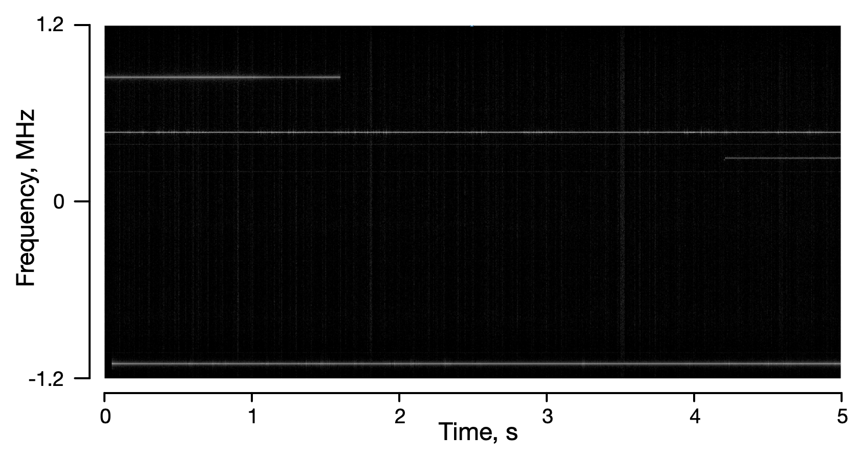
The frequencies are relative to the carrier frequency. You can see the ATIS signal tha appears continuously, and then three other signals that are appearing or ending.
What we want to be able to do is figure out which frequency each signal is at, so that we can demodulate them, and listen to them as we did last time. If we wanted to extract the signal at about -1.1 MHz, it would be good to know exactly where it is. The signal is there at 1 second, which is 2.4e6 samples into the data. If we want to measure the frequency to 1 kHz, we need 100 ms of data which is 1/ 1 kHz, or 2400 samples. We can plot this with
>>  % desired frequency resolution
>>  freq_res = 1000;
>>  % number of samples needed at a sampling rate of fs
>>  n_samp = fs/freq_res;
>>  % start time, seconds
>>  t0 = 1;
>>  % starting index, seconds times sampling rate
>>  n0 = t0 * fs;
>>  % spectrum of a segment of the signal
>>  d2f = fftshift(fft(d2(n0+1:n0+n_samp)));
>>  % frequency axis
>>  f = [-n_samp/2:n_samp/2-1]*freq_res;
>>  % Plot the spectrum
>>  plot(f,abs(d2f));
The result is
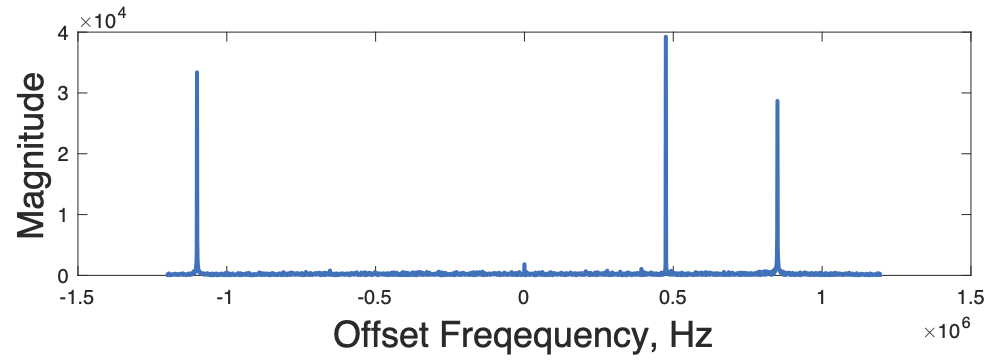
We see all three peaks that we saw above. The question now is exactly what are the frequecies. We can find the maximum signals location with
This is the maximum value, and the sample where it occurs. To find the offset frequency in Hz, we just need to multiply by the frequency resolution. To find the actual frequency to set the receiver to, add the 134.8e6 frequency of the carrier.
>> d2f_offset = (dndx - n_samp/2)*freq_res

d2f_offset =

      476000

>> d2f_cf = d2f_offset + fc

d2f_cf =

   135276000
The subtraction of half the frame size, fr/2, corrects for the fact that the zero frequency in the spectrum is in the middle.
We can then use the offset frequency the same as lat week to demodulate that signal and play it back. Or we could start up gqrx and set it to 135.276e6 Hz, and see what is there. This happens to be the Palo Alto ATIS.
To find the peaks of the other signals we can do
These are all of the signals that are above 10\% of the peak signal we found above. There is one around 101, the the ATIS signal above at 1678, and another at 2051. We can compute the offset frequency for each of these, and demodulate and decimate them to play back just that channel.
Your Lab Report
Your task will be to automate the proess, so that you can automatically find the frequencies of interest in a signal, and play them back.
-
Write an m-file function that takes one of the data sets, and plays back the entire band, as we did above. You can assume the basic parameters (sampling rate, etc). Have it return the audio waveform.
For your report, include a plot of the audio for one of the data sets we haven't looked at so far, or of one of your own. Also include your m-file.
-
Write an m-file to find the interesting signals in a data file. Since the signals come and go, you want to check a couple times a second to see if anything has appeared. It should return the frequencies (both offset frequencies and the actual carrier frequency you would use with gqrx or sdrsharp).
For your report, include the frequencies and times you found for one of the other data files. Again, include your m-file.
-
Write an m-file function that automatically scans through a data file, and extracts the signals it finds.
For your report, include a plot of the extracted signals, as well as your m-file.