Lab 4: Narrowband FM
Overview
For the last wo weeks we have been learning how to find AM signals, and then demodulate and decimate them down to a baseband signal you could listen to. For AM simply taking the absolute value of the complex signal detects the envelope, and gives you the audio waveform.
This week we will look at narrowband FM (NBFM). Finding the signals and the initial demodulation and decimation process are the same as for AM. The difference lies in how you detect the message in the FM signal. We will implement a simple method for this, and listen to narrowband FM traffic on the amateur radio VHF band.
Aims of the Lab
The goal of this lab is to learn how to detect messages in narrowband FM signals.
Narrowband FM Signals
Narrowband FM is commonly used in Amateur Radio in the 144--148 MHz VHF band and the 420--450 MHz UHF band, where the bandwidth required for the FM signal is acceptable. It was also commonly used for Police, Fire, and Emergency Services, but these have mostly gone to digital systems that we will talk about later. You can also find a number of Stanford groups that use narrowband FM, such as Athletics and RDE.
We'll start with the VHF Amateur Radio band. The following file is a capture of 2.4 MHz of the RF spectrum centered at 145 MHz.
The upper end (well actually, most) of the VHF amateur band is allocated to FM repeaters. These are moderately powerful radios (50W) located in high places that listen on one frequency and transmit on another. In the VHF band this offset is +/- 600 kHz, which is far enough apart to allow the repeater to listen and transmit at the same time. The offset is +/- 5 MHz in the UHF band, where more spectrum is available.
Repeaters are important because radio communications in the VHF band (and above) are essentially limited to line of sight. This isn't very far when hills and buildings are in the way. However, repeaters are located in high places like the tops of mountains. If you and the person you want to communicate with can see the same repeater/mountain, you can talk to each other. This allows people in large areas to communicate.
One of the most active repeaters in the valley is N6NFI, operating at a transmit frequency of 145.230 MHz. This repeater is located right above Stanford on the south end of the hill with the Dish. If you walk the Dish path starting at Stanford Avenue, the N6NFI antenna is one of the antennas located on the left shortly after you reach the top of the hill. Someone is talking on this channel most of the day. The busiest time is from 9 AM to about 11 AM, when the "9 O'Clock Net" is happening. People call in to talk about all sorts of things, radio related and otherwise. If you want to get people going, call in and ask what "ground" really means!
The captures were taken at the start of the 9AM net. The acquisition parameters were largely the same as for the AM airband signals from Lab 3. Only the center frequency was changed
>>  % center Frequency, VHF amateur radio band
>>  fc = 145.0e6;
>>  % Sampling Frequency
>>  fs = 2.4e6;
>>  % frame size
>>  fr = 240e3;
>>  % Number of frames
>>  nf = 200;
>>  % Gain
>>  g = 30;
>>  tn1 = Read_RTLSDR(fc,fs,fr,nf,g);
The variables fc, fs, fr, nf, and g are included along with the data. The data is in tn1, tn2, or tn3, depending on the file.
This is what the activity looked like on GQRX
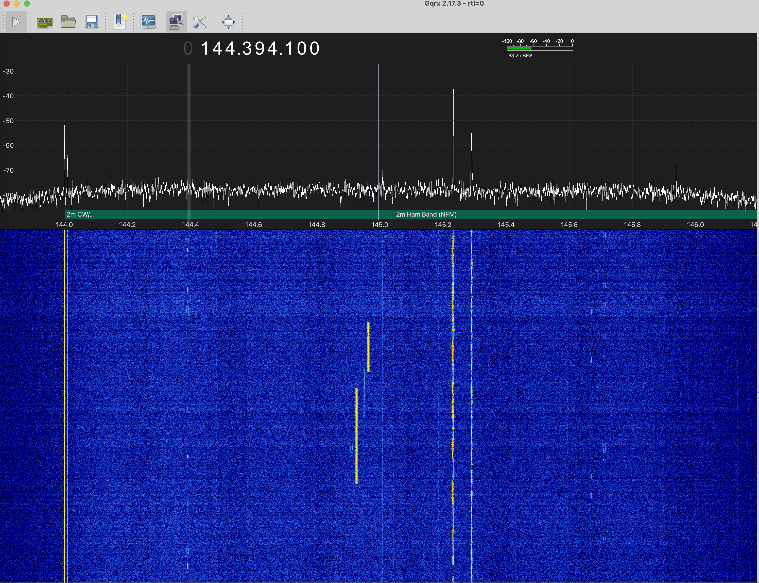
You see a number of different signals. The one we are after is 145.23 MHz, which is slightly to the right of center. It is the strongest signal present. You also see another narrowband FM station at a slightly higher frequency, The two bright signals lower down are digital DStar repeaters. You also see a number of packets. The ones just below 144.4 MHz are a digital packet radio protocol called APRS. We may look at this later in the class. The signals at 144 MHz are just interference.
Load a data file, and see if you can find the frequency offset for the N6NFI repeater. It is the strongest signal in the data, so it should be pretty obvious. Find the offset of the frequency of the strongset signal, just as you did in Lab 3. Demodulate the signal, and decimate it by a 120. This will leave you with a signal sampled at 2.4 MHz/ 120 = 20 kHz. This is a wider bandwidth than the signal requires, but this makes the demodulation easier. We'll decimate once more at the end.
I'm assuming you are starting with tn1, demodulate it to baseband as tn1m, and then decimate it to tn1md. Substitue your own variable names as needed.
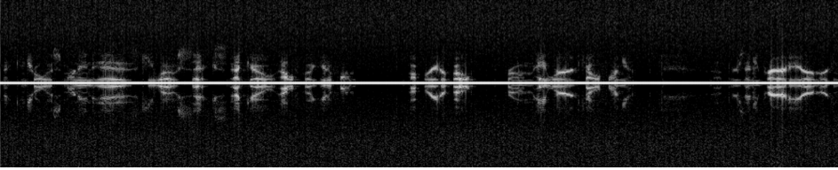
If you plot the spectrogram of the resulting demodulated and decimated signal tn1md,
you should see something like this
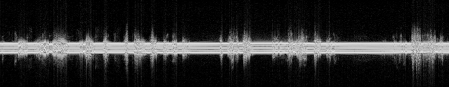
Clearly there is information there.
If you plot the magnitude of the signal,
>> % Time axis after decimation
>> ts = t(1:120:end);
>> plot(ts, abs(d1md))
>> xlabel('Time, s');
>> ylabel(Magnitude');
it should be almost constant.
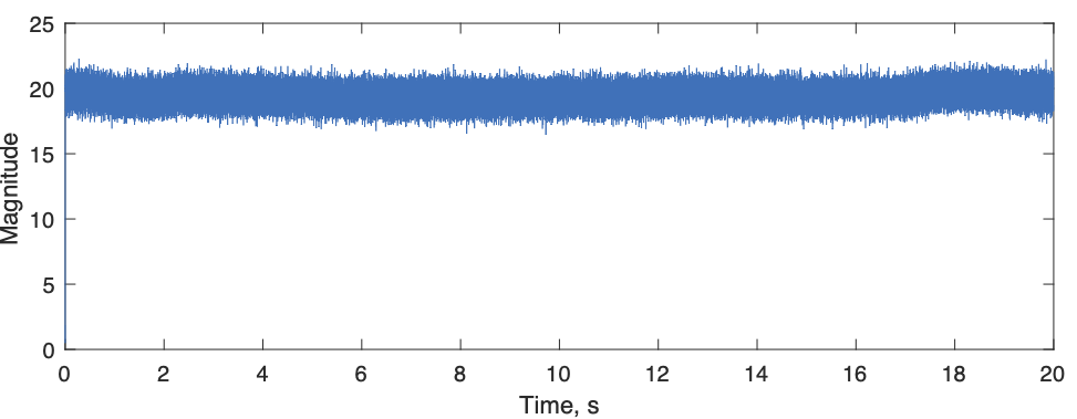
This is because all of the information is in the phase.
Decoding Narrowband FM Signals
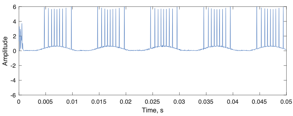
From class, the way you would expect to extract the audio waveform from the FM signal would be to differentiate the angle of the signal
This doesn't work very well, although it can be fixed up. The first part of the signal shows what the problem is
A better idea is to detect the message from the FM signal with this
You will take a look at what this does and why it works in your lab report.
An even simpler version replaces the angle() operation with taking the imaginary part with imag(). Try this. Why does this work?
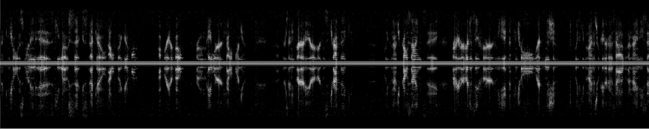
The spectrogram of the resulting signal now should look like this
This is a very nice voice audio spectrum.
You can see that the signal is narrower bandwidth than we need, so we'll decimate it once more
The spectrogram now looks like
To compare the two, play them through your sound card
Both should have very clear audio, much clearer than the AM signal from last week. The second one has much less static.
Sometimes you will want to interrupt the sound output. The trick is to
This resets the whole sound system. Nothing else seems to work.
The clear audio is the reason FM is so widely used. If the signal is above a threshold so that the phase can be accurately determined, the result is essentially perfect audio. The price for this is that the transmitter is putting out a full amplitude frequency modulated sinusoid continuously no matter what the input is. This requires even more power than AM. However, the amplifier doesn't need to be linear if the harmonics are filtered out after the output stage. This allows FM amplifiers to be much less expensive than linear AM amplifiers, so the overall cost of an FM transmitter can be much less than for an AM transmitter of the same power and frequency.
One of the things you hear in the audio is a background hum. You can also see it in the spectrogram as two continuous frequency lines on either side of DC. This sounds and looks like an artifact, but is actually put there on purpose. One of the problems with repeaters is that they retransmit everything they hear at their receive frequency. This could be noise or interference, or even another repeater. To solve this repeaters only retransmit signals if they contain a specific tone. This indicates that the signal was intended for them, and should be retransmitted. The tones are chosen to be "sub-audible" around 100 Hz, but clearly you can hear them. Some repeaters suppress the tone when they retransmit a signal. N6NFI does not, as you can hear.
The tone is called a CTCSS code for "Continuous Tone Coded Squelch System", or more commonly as a PL code for Motorola's trademark name "Private Line". There are also lots of other access methods that use digital codes, tone bursts, or tones at higher frequencies. These are less common.
Use a segment from the data to determine what the CTCSS frequency is for N6NFI. The audio signal a1d is sampled at 10 kHz. If we compute the spectrum of 1000 samples, we would have 10e3/2000 = 10 Hz resolution. Compute the spectrum, and determine how many samples away from the carrier the CTCSS tone is. Look it up on the web (google "N6NFI and CTCSS") to see if you are right.
Odd Fact
Try your AM receiver m-file on a narrowband FM signal. Why does this work at all? It works better as the AM receiver bandwidth is narrowed, and as you move slightly off the transmit frequency.
Lab Report
For the lab report you can use the other captures listed above. You can also capture a signal yourself. Here are a couple more to consider
This has a set of channels giving the weather at points around the bay area. These are nice strong clean signals, and you can choose any of them.
1. Make a Narrowband FM Receiver
Starting from your AM receiver from Lab 3, modify the demodulator to work for narrowband FM. Choose one of the other amateur band signals or the weather radio signals and demodulate them.
Look for the strongest signals, like last time. Skip the first 2000 samples, though, there is a transient where the receiver is getting going.
a) What was the offset frequency for the signal?
b) Plot the magnitude of the demodulated and decimated FM signal to show that it is essentially constant. There will be some noise, but it turns out that noise in the magnitude has very little effect on the detected FM signal. Why is that?
c) Provide a screen capture of the spectrogram of the decoded baseband audio signal.
2. FM Demoduation
We looked at two different ways to decode the FM signal.
a) What is the problem with using diff(angle(baseband_signal)) to decode the FM signal?
b) How does the approach proposed above work?
c) Why can the angle operation be replaced with taking the imaginary component, and have it still work?
3. Finding the CTCSS Frequency
What is the CTCSS frequency for N6NFI? This is the constant tone you hear when there is no other signal present. You just want to make an estimate of its frequency.
This clip will help you check your answer:
4. Suppressing the CTCSS Tone
Design a highpass filter that suppresses the CTCSS tone. The filter should have a half amplitude bandwidth of +/- 150 Hz, and have a transition width of about 100 Hz.
a) First design a lowpass filter that just passes the CTSS tones. This will be a windowed sinc, where the length is determined by the transition width, as described in class. The number of samples in the filter is the length of the filter in time multiplied by the sampling rate. Include a plot of the filter impulse response.
b) Design a matching highpass filter by first normalizing the lowpass to have a total area of 1. Then subtract your filter from a unit impulse at zero, which is the middle of the filter.
Plot the frequency response to make sure it is doing what you expect.
c) Filter the demodulated signal with
Plot the first 1000 samples of the signal before and after filtering. This will show that the CTCSS tone is really gone. Submit a screen capture of the spectrogram. When you listen to the resulting signal it should much better with the CTCSS tone gone!
My filter ended up with about 200 samples, and a time-bandwidth product of 6.
5. Using an AM receiver on an FM signal
Why does using your AM receiver on an FM signal work at all? This is a non-trivial question, so any reasonable answer will be accepted.