K-nearest neighbors
Contents
\(K\)-nearest neighbors#

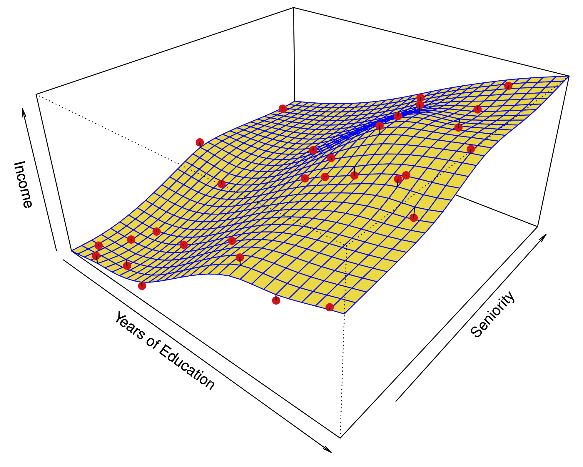
Fig. 15 Illustration of KNN regression: \(K=1\) (left) is rougher than \(K=9\) (right)#
KNN estimator#
Comparing linear regression to \(K\)-nearest neighbors#
Linear regression: prototypical parametric method. Easy for inference.
KNN regression: prototypical nonparametric method. Inference less clear.
Long story short:#
KNN is only better when the function \(f\) is far from linear (in which case linear model is misspecified)
When \(n\) is not much larger than \(p\), even if \(f\) is nonlinear, Linear Regression can outperform KNN.
KNN has smaller bias, but this comes at a price of higher variance.
KNN estimates for a simulation from a linear model#

\(K=1\) on left, \(K=9\) on right.
Linear models can dominate KNN#

Truth is linear, plot of test MSE vs. 1/K shows KNN worse than linear regression.
Increasing deviations from linearity#

When there are more predictors than observations, Linear Regression dominates#

When \(p\gg n\), each sample has no near neighbors, this is known as the curse of dimensionality.
The variance of KNN regression is very large.

