Experimental data evaluation

A total of 146 combustion property targets were selected for model optimization and uncertainty minimization.  They include laminar flame speeds, shock tube ignition delays, and species profiles determined in flow reactors and shock tubes. In FFCM-1, the fuels or reactants considered are H₂, CO, CH₄, CH₂O, C₂H₆, and H₂O₂. 

To assess the experimental target uncertainty in a systematic manner, statistical analysis of the data scatter was made. We highlight some of these analyses here.

Laminar Flame Speed
A rational function analysis [1] was made for the laminar flame speed where repeated measurements were available across different techniques and laboratories.  Figure 1 shows an example of a 6-parameter rational function analysis for the CH₄/air flame speed at 298 K and 1 atm.  The range of the 95% confidence interval is taken to be ±2σ bounds.  Similar analyses were made for the flame speeds of H₂-air mixtures, 50%CO-50%H₂-air mixtures, 95%CO-5%H₂-air mixtures, C₂H₆-air mixtures, all at 298 K and 1 atm, and methane-air mixtures at 298 K and 2 atm.

In general, the scatter uncertainty in the flame speed value is positively correlated with the magnitude of the flame speed.  As shown in Figure 2, the data uncertainties given by the rational function analysis increases with an increase in the flame speed value.

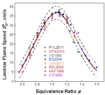
Figure 1. Rational function analysis with uncertainty bounds for CH₄/air laminar flame speed at 298 K and 1 atm. Symbols: experimental data; solid line: nominal fit; dashed lines: 95% confidence interval.  Data references can be found on the Optimization/Performance page.

 

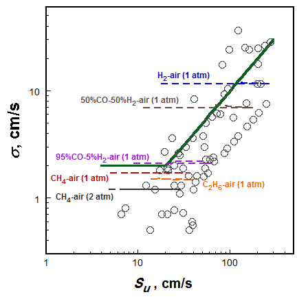
Figure 2. Dependence of uncertainty on the mean flame speed value given by the rational function analysis (dashed lines), compared to uncertainties reported for each measured flame speed value (symbols).  The solid line represents the evaluated uncertainty of all flame speed data for which the data sample size is too small for an appropriate uncertainty analysis.

 

Individually reported experimental uncertainties are also presented, showing the trend and magnitude similar to the results of rational function analysis.  Keeping in mind that the individually reported experimental uncertainty values do not consider systematic uncertainties, we assigned the uncertainty of those flame speed data that cannot be statistically analyzed to be $\max(2 cm/s, 10\%S_u)$, i.e., the solid line shown in Figure 2.

Shock-Tube Ignition Delay
Shock tube target data scatter uncertainties were analyzed in a similar manner.  Figure 3 shows such an analysis using the data of Seery and Bowman [2] as an example.  Experimental data of the same source and similar compositions and conditions are analyzed together with empirical function $\tau=A[fuel]^\alpha[oxidizer]^\beta[diluent]^\gamma \exp(B/T)$. This way we have large enough datasets for statistical analysis. The mean value and the upper and lower bounds showing 95% confidence interval are shown with solid lines.

 

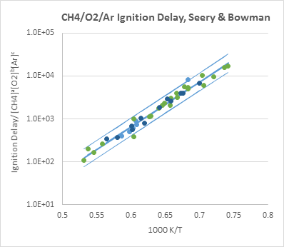
Figure 3. A sample empirical function analysis of shock tube ignition delay data. The middle line represents the mean and the upper and lower lines are ±2σ uncertainties.

 

Shock-Tube Species Profiles
For shock tube species concentration and cases where only a few data points are available, scatter uncertainty was estimated to be caused by temperature scatter and target definition. Temperature scatter can be obtained from the Arrhenius plot of a certain measurable (e.g., rate constant), which usually accompanies species profile measurements. Scatter uncertainty in species profile caused by temperature scatter is then modelled by adding temperature perturbation in computational tests. Uncertainty from target definition comes from the difficulty to locate the peak, etc., and was also estimated from modeled profile. For example, if a target is defined as the time to maximum mole fraction of a species such as OH or CH₃, the ±2σ uncertainty is approximated by the time period for which the species mole fraction exceeds 95% of its peak value, because of difficulties in precisely pinpoint the maximum mole fraction value. Targets defined as "time to 50% of the maximum concentration of OH or CO" were treated similarly, with the time period between 45% and 55% taken as ±2σ range.

Initial Conditions in Shock-Tube and Flow Reactor Experiments
Special attention was placed on the assessment of the uncertainties in the initial conditions and their impact on the simulation of flow reactor and shock tube experiments.  Shock tube experiments can be sensitive to less than ~1 PPM initial impurities [3]. Shock-tube data, including ignition delay times and species profiles, are excluded from consideration when calculations show a marked sensitivity of the response towards 1 PPM of H atom. Examples of ignition delay time sensitive to initial impurities include Cheng & Oppenheim, 1984 [4] and the TAMU and DLR measurements reported in Kéromnès et al., 2013 [5]. Figure 4 shows an example of an excluded target, which is found to be extremely sensitive to the presence of initial impurities. Adding 1 ppm of H atoms into a 3.46% H₂ / 3.49% O₂ / Ar mixture at an initial temperature of 998 K and pressure of 3.99 atm can cause the ignition delay time, defined as time to maximum OH* mole fraction, to decrease by as much as 90%. Clearly, the problem is particularly severe for hydrogen ignition experiments near the second explosion limit. We exclude the ignition targets of Davis et al. [6] and those of more recent studies that have significant impurity sensitivities. The list of excluded targets is given in Table 1, along with the results of impurity sensitivity tests. For targets that have acceptable impurity sensitivity but do not have a reasonable assessment of initial impurity effects, the modeled difference caused by 1 ppm H atom addition was estimated to provide the 2σ impurity uncertainty for that experiment. Uncertainty resulting from error or variation in the initial temperature was also estimated by modeling. In all cases, the uncertainty in the temperature behind reflected shock waves is assumed to be ±10 K.

The overall uncertainty of shock tube targets was estimated from the above sources by adding the different factors in quadrature.

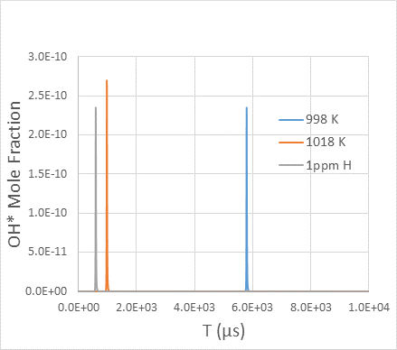
Figure 4. Example of an abandoned target that shows extreme sensitivity to 1 PPM H atom addition (initial impurities) and initial temperature perturbation. Blue line: model prediction for the nominal case (3.46% H₂ / 3.49% O₂ / Ar mixture at an initial temperature of 998 K and pressure of 3.99 atm); orange line: with +20 K temperature perturbation; grey line: with 1 ppm H atom addition to the initial mixture.

Table 1. Excluded H₂ ignition delay targets from [6] and some of the more recent studies.

T (K)	p (atm)	Nominal Prediction (μs)	With 1 ppm H Atom (μs)	Description	Reference
1051	1.719	378	184	6.67%H2/3.33%O2/90%Ar	[4]
1312	2.008	66.0	45.6	6.67%H2/3.33%O2/90%Ar	[4]
1033	0.518	390	210	20%H2/10%O2/70%Ar	[7]
1510	0.493	38.4	33.0	20%H2/10%O2/70%Ar	[7]
1102	3.393	242.9	121.8	4%H2/2%O2/94%Ar, dp/dt=5.93%/ms	[8]
958	3.706	7815	4135	4%H2/2%O2/94%Ar, dp/dt=2.08%/ms	[8]
1035	15.86	7307	4691	0.0346H2/0.0349O2/0.9305Ar	[9]
998	3.99	5793	599	0.0346H2/0.0349O2/0.9305Ar	[9]
950	0.926	2065	806	0.0346H2/0.0349O2/0.9305Ar	[9]
1100	14.5	922.9	449.5	0.0587H2/0.0295O2/0.9118Ar	[9]
1020	3.51	641.9	198.2	0.0587H2/0.0295O2/0.9118Ar	[9]
961	0.89	1767.8	730.7	0.0587H2/0.0295O2/0.9118Ar	[9]

 

Accurate simulation of flow reactor experiments is complicated by several factors, especially when the reactor operates neither adiabatically nor isothermally.  As Figure 5 shows, the measured temperature lies between what can be predicted by an isothermal model and an adiabatic model. The computation here was carried out using the FFCM trial model.  Additionally, simulation also shows two characteristic behaviors generic to all other flow reactor data on H₂ oxidation—(a) while the oxidation rate computed for the isothermal model is slow compared to the experimental data, the rate computed with the adiabatic model is too fast; (b) the computed species profiles need to be shifted to match the onset of reaction, unless some free radicals are introduced artificially at time zero.  The first problem represents heat loss in the experiment not accounted for by the model.  The second problem reflects the fact that the reactor cannot set absolute zero reaction time because of radical production possibly in the mixer or heating region. (Time shifting of the model to accommodate pre-reaction is most often used, but is poorly suited for including this lower temperature data in optimization. Other methods include model initialization with measured key species or with introduction of an adjustable initial radical concentration. [10])

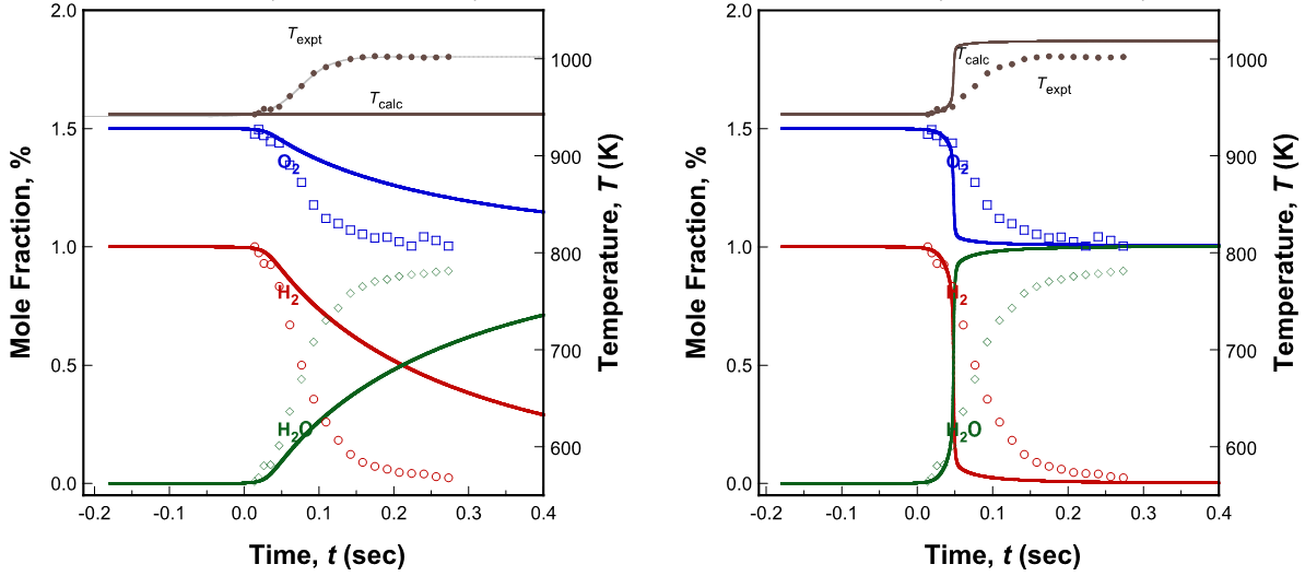
Figure 5. Experimental (symbols) and computed (lines: FFCM trial model) species profiles during the oxidation of hydrogen in oxygen-nitrogen at 2.5 atm in the Princeton flow reactor.  The initial reactant composition is 1% H₂-1.5%O₂. Left panel: isothermal; right panel: adiabatic.

Our way to solve these problems is to use measured temperature profiles in the simulation and to assume a certain free-radical concentration at time zero. The experimental temperature-time history may be fitted into a hyperbolic function of the form T(t) = T_a + a tanh[b (t - c)], where T₀, a, b and c are fitting parameters.  The time derivative of the above function is dT/dt = ab [1 – tanh²(b (t - c))], with T(0) = T_a + a tanh(-bc).

Figure 6 shows the simulation results obtained with the temperature-time history imposed by the above equation, comparing cases with/without the presence of a radical at time zero.  Without initial free radicals, the simulation results show an abrupt change in the species concentrations around 0.1 sec into the reaction. This species time history is inconsistent with the temperature profile. The rise in temperature is gradual, indicating gradual heat release consistent with the gradual change in the measured species profiles.  These profiles are reproduced only when a free radical was introduced artificially at time zero.   Figure 6 shows that for this specific experiment the species profiles are reproduced well with 10 PPM OH at time zero without having to assume time shift and in fact, the same quality of agreement can be achieved with any free radicals introduced at time zero.

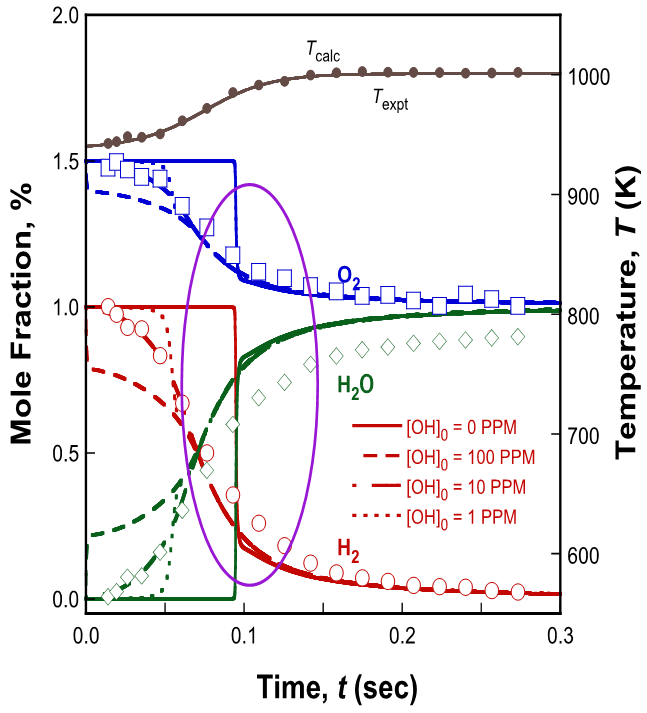
Figure 6. Experimental (symbols) and computed (lines: FFCM trial model) species profiles during the oxidation of hydrogen in oxygen-nitrogen at 2.5 atm in the Princeton flow reactor.  The initial reactant composition is 1% H₂-1.5%O₂. The computation used the experimental temperature profile as the input.

Given the sensitivity of the species concentration profile to the radical input at zero time, OH radical concentration was adopted as an additional active parameter.  Figure 7 shows an example of prediction with added OH radical, at its nominal concentration as well as its upper and lower bounds.

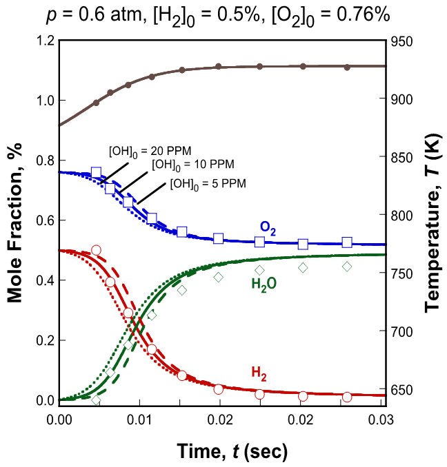
Figure 7. Determination of nominal value and bounds of initial radical concentration.

References

[1] Law CK, Wu F, Egolfopoulos FN, Gururajan V, Wang H. On the Rational Interpretation of Data on Laminar Flame Speeds and Ignition Delay Times. Combust Sci Technol. 2015;187:27-36.
[2] Seery DJ, Bowman CT. An experimental and analytical study of methane oxidation behind shock waves. Combust Flame. 1970;14:37-47.
[3] Urzay J, Kseib N, Davidson DF, Iaccarino G, Hanson RK. Uncertainty-quantification analysis of the effects of residual impurities on hydrogen–oxygen ignition in shock tubes. Combust Flame. 2014;161:1-15.
[4] Cheng RK, Oppenheim AK. Autoignition in methane–hydrogen mixtures. Combust Flame. 1984;58:125-39.
[5] Kéromnès A, Metcalfe WK, Heufer KA, Donohoe N, Das AK, Sung C-J, Herzler J, Naumann C, Griebel P, Mathieu O. An experimental and detailed chemical kinetic modeling study of hydrogen and syngas mixture oxidation at elevated pressures. Combust Flame. 2013;160:995-1011.
[6] Davis SG, Joshi AV, Wang H, Egolfopoulos F. An optimized kinetic model of H₂/CO combustion. Proc Combust Inst. 2005;30:1283-92.
[7] Cohen A, Larsen J. Explosive mechanism of the H₂-O₂ reaction near the second ignition limit. Aberdeen (MD): Ballistics Research Laboratories; 1967. Report No. 1386.
[8] Pang GA, Davidson DF, Hanson RK. Experimental study and modeling of shock tube ignition delay times for hydrogen–oxygen–argon mixtures at low temperatures. Proc Combust Inst. 2009;32:181-8.
[9] Herzler J, Naumann C. Shock-tube study of the ignition of methane/ethane/hydrogen mixtures with hydrogen contents from 0% to 100% at different pressures. Proc Combust Inst. 2009;32:213-20.
[10] Zhao Z, Chaos M, Kazakov A, Dryer FL. Thermal decomposition reaction and a comprehensive kinetic model of dimethyl ether. Int J Chem Kinet. 2008;40:1-18.