Response Surface

Response surfaces are used in the MUM-PCE procedure [1] to reduce computation time. In the FFCM work, second-order polynomials are used. $$\eta_r(\mathbf x)=\mathbf a^T \mathbf x + \mathbf x^T \mathbf b \mathbf x $$ In the above equation, $\eta_r(\mathbf x)$ is the response, $\mathbf x$ is the active parameter vector, and $\mathbf a$ and $\mathbf b$ are the coefficient arrays. A traditional way to obtain response surface coefficients is by the factorial test of computational experiments [2]. Other approaches include sensitivity analysis-based method (SAB) [3] and Monte Carlo (MC) simulation.

Response surface of an ignition delay target is used to test the accuracy of different approaches. Methods of MC and factorial computational experiments are compared with the SAB method, as shown in Figure 1. The SAB method is shown not to give satisfactory results. The surface generated by the factorial training set performs well on the factorial points but does not give satisfactory results for the interior MC points. The surface generated from the MC training set exhibits the opposite tendency. Combination of the factorial and MC points provides better overall results than factorial or MC alone. Increasing number of MC points further does not show significant improvement.

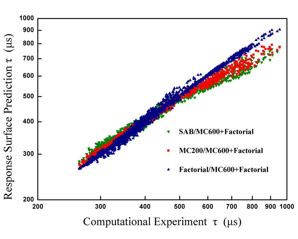
Figure 1. 45-degree diagonal plot of response surface accuracies. Tests were made for 600 MC plus full, 2ⁿ factorial points, comparing response surfaces constructed with the SAB method, the factorial design, and 200 MC points.

In the FFCM-1 work, response surfaces are sometimes generated from a combination of factorial design and MC analysis. Most targets have a too large number of active parameters, rendering the factorial design method inefficient. Their response surfaces have to be generated from MC simulations.

Figures 2 thru 6 are samples of accuracy tests of response surfaces. Uncertainties from response surfaces are usually substantially smaller than the uncertainties in the corresponding targets.

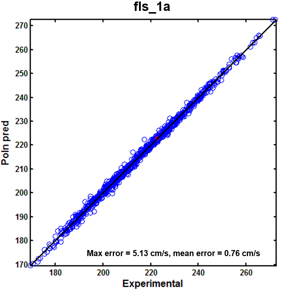
Figure 2. Response surface predictions versus computational experiment values for a typical flame speed target.

Figure 3. Response surface predictions versus computational experiment values for a typical ignition delay target.

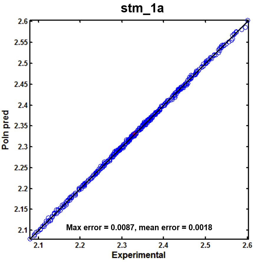
Figure 4. Response surface predictions versus computational experiment values for a typical shock-tube time corresponding to a particular concentration value of a species.

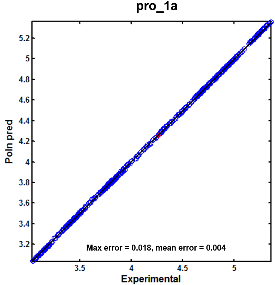
Figure 5. Response surface predictions versus computational experiment values for a typical shock-tube species concentration.

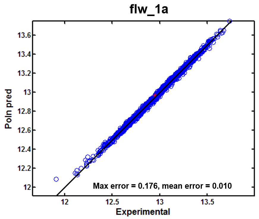
Figure 6. Response surface predictions versus computational experiment values for a typical flow reactor species concentration.

References

[1]  Sheen DA, Wang H. The method of uncertainty quantification and minimization using polynomial chaos expansions. Combust Flame. 2011;158:2358-74.

[2]  Frenklach M, Wang H, Rabinowitz MJ. Optimization and analysis of large chemical kinetic mechanisms using the solution mapping method—combustion of methane. Prog. Energy Combust. Sci. 1992;18:47-73.

[3]  Davis SG, Mhadeshwar AB, Vlachos DG, Wang H. A new approach to response surface development for detailed gas‐phase and surface reaction kinetic model optimization. Int J Chem Kinet. 2004;36:94-106.