Syllabus
Contents
Syllabus#
Videos: Every lecture will be recorded by SCPD
Email policy: Please use the Piazza site for most questions. For administrative issues that only concern you, email the course staff mailing list: stats202-aut2021-staff@lists.stanford.edu
Website: stats202.stanford.edu
If you are auditing the class (not registered on Axess), email us your SUNet ID in order to gain access to the lectures and homework on canvas.
Prediction challenges#
The MNIST dataset is a library of handwritten digits#
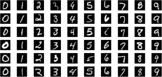
MNIST dataset#
In a prediction challenge, you are given a training set of images of handwritten digits, which are labeled from 0 to 9.
You are also given a test set of handwritten digits, which are not identified.
Your job is to assign a digit to each image in the test set.
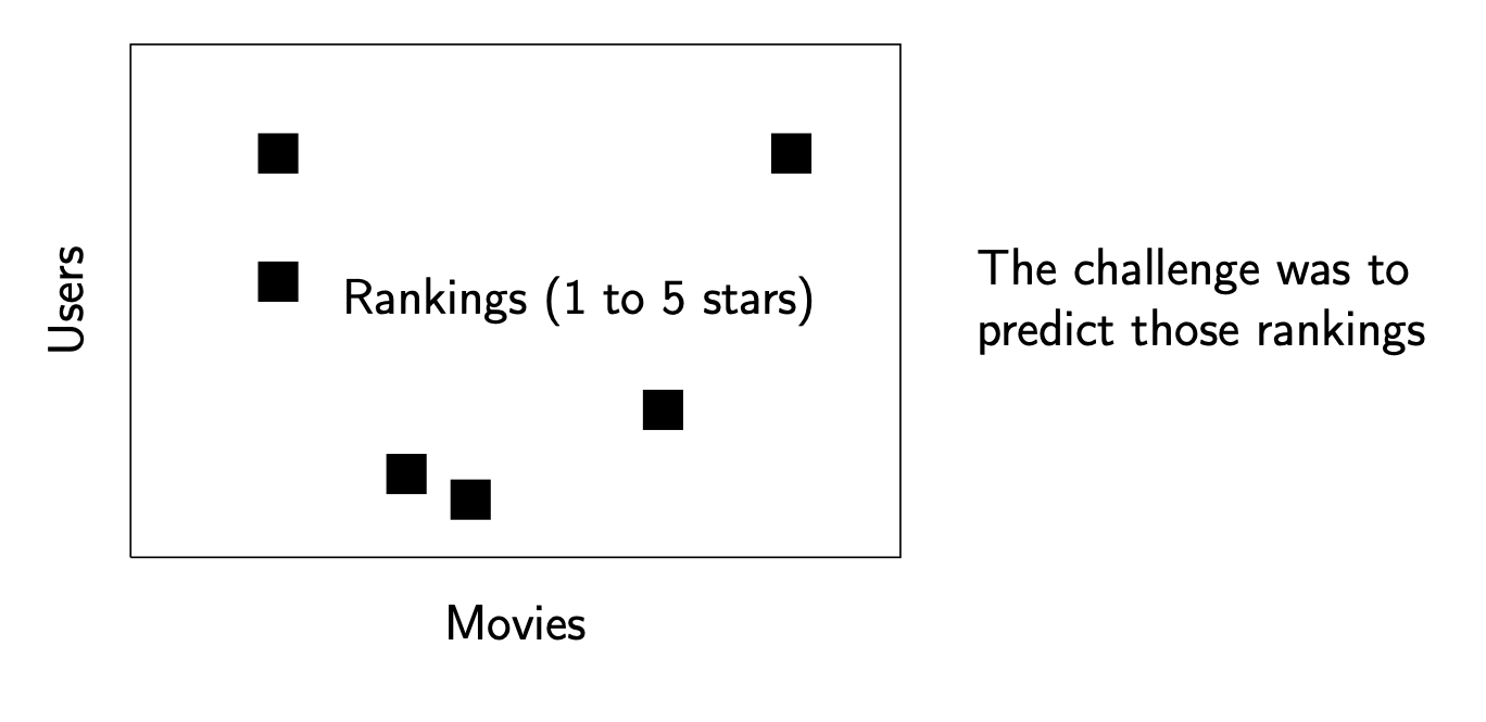
The Netflix prize#
Netflix popularized prediction challenges by organizing an open, blind contest to improve its recommendation system.
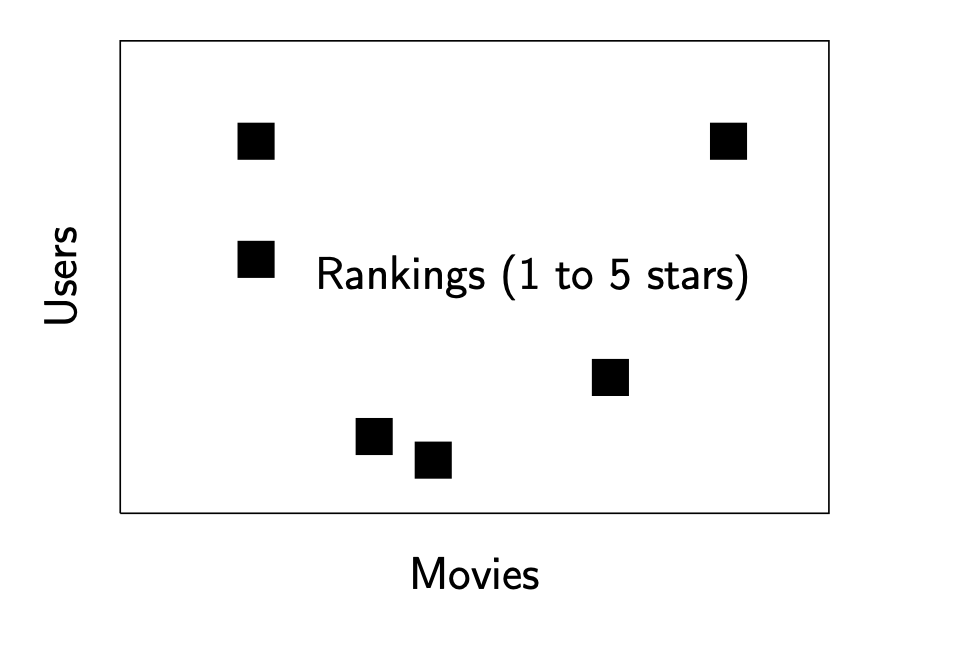
Netflix 1#
The Netflix prize#
Netflix popularized prediction challenges by organizing an open, blind contest to improve its recommendation system.
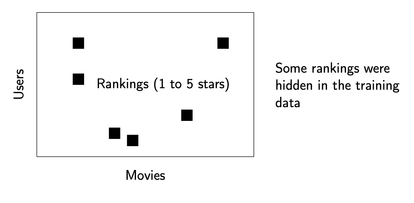
Netflix 2#
The Netflix prize#
Netflix popularized prediction challenges by organizing an open, blind contest to improve its recommendation system.
Netflix 3#
The prize was $1 million.
(Cue Dr. Evil jokes if anyone knows Austin Powers movies…)
Unsupervised learning#
In unsupervised learning we start with a data matrix:
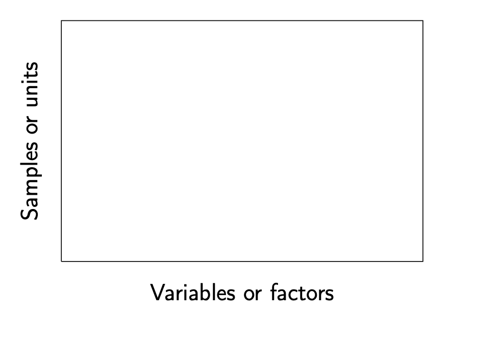
Unsupervised learning setup#
Quantitative, eg. weight, height, number of children, …;
Qualitative, eg. college major, profession, gender, …;
Goals of unsupervised learning#
In unsupervised learning we start with a data matrix:
Our goal is to:
Find meaningful relationships between the variables or units: Correlation analysis.
Find interpretable low-dimensional representations of the data which make it easy to visualize the variables and units. PCA, ICA, isomap, locally linear embeddings, etc.
Find meaningful groupings of the data. Clustering.
Unsupervised learning is sometimes referred to in Statistics as exploratory data analysis.
Supervised learning#
Setup#
In supervised learning, there are input variables, and output variables:

Classification problems#
In supervised learning, there are input variables, and output variables:

Goals of supervised learning#
In supervised learning, there are input variables, and output variables:
If \(X\) is the vector of inputs for a particular sample. The output variable is modeled by: $\(Y = f(X) + \underbrace{ \varepsilon}_{\text{Random error}}\)$
Our goal is to learn the function \(f\), using a set of training samples \((x_1,y_1)\dots(x_n,y_n)\)
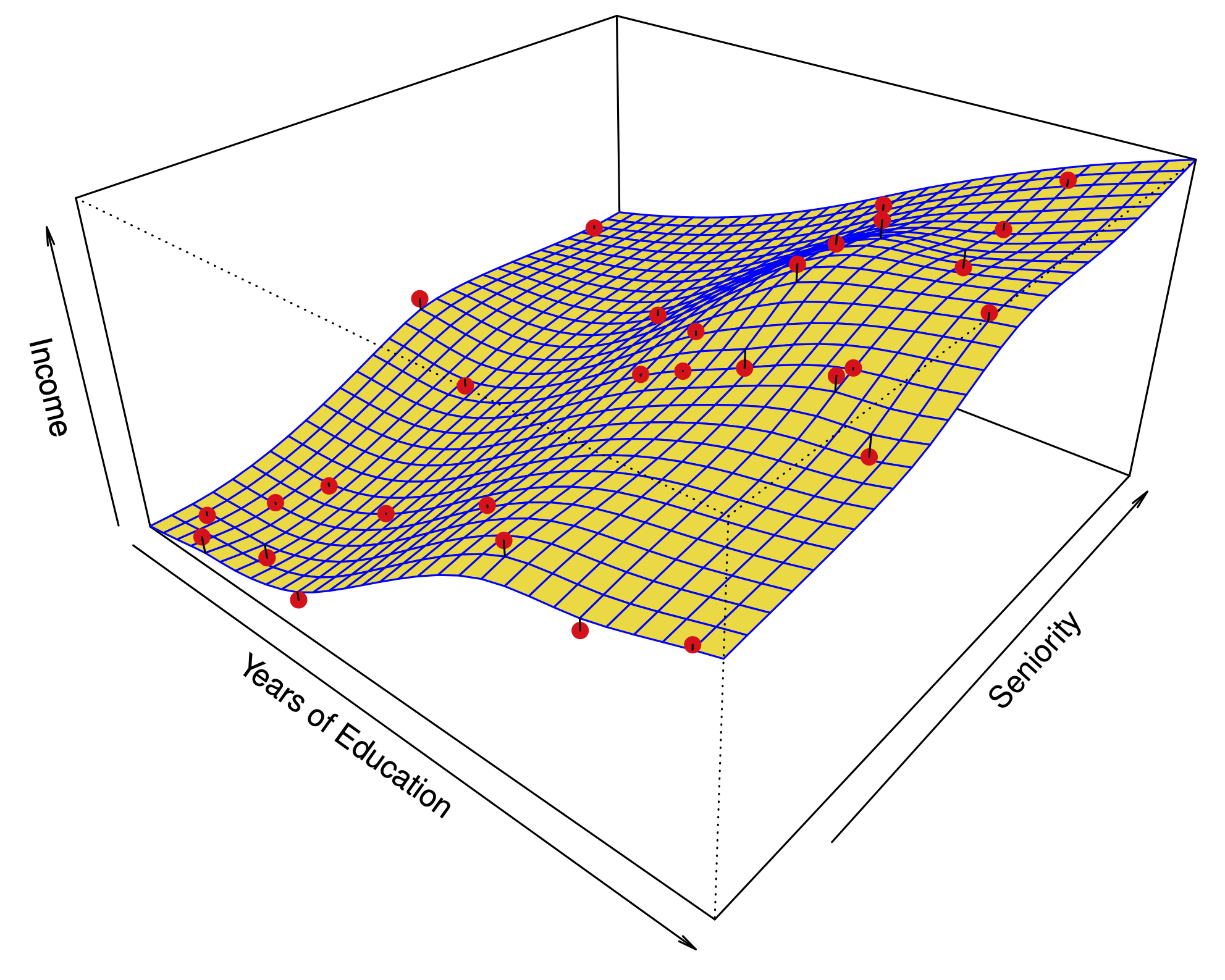
Regression model#
Motivations#
| **Prediction:** Useful when the input variable is readily available, but the output variable is not. | Example: Predict stock prices next month using data from last year. |
| **Inference:** A model for $f$ can help us understand the structure of the data --- which variables influence the output, and which don't? What is the relationship between each variable and the output, e.g. linear, non-linear? | Example: What is the influence of genetic variations on the incidence of heart disease. |
Kaggle: data analysis competitions#
Business model#
Organize prediction competitions hosted online.
Offer companies consulting services from Kaggle ``stars’’.
Kaggle-in-class is a competition engine offered to degree-granting institutions for free. Stats 202 was the first class to use it (or so I’m told)!
Kaggle: data analysis competitions#
A sample Kaggle challenge#
Help out San Francisco’s foremost Baroque ensemble bring in subscriptions!
Using Philharmonia’s database of subscriptions and single ticket sales, including information about concerts, and patrons, predict who will subscribe for the 2021-2022 season.
Create an interactive visualization of Philharmonia’s database using the R package Shiny.
This year’s competition coming soon!
Parametric and nonparametric methods#
There are (broadly) two kinds of supervised learning method:
Parametric methods: We assume that \(f\) takes a specific form. For example, a linear form: $\(f(X) = X_1\beta_1+\dots +X_p\beta_p\)\( with parameters \)\beta_1,\dots,\beta_p$. Using the training data, we try to fit the parameters.
Non-parametric methods: We don’t make any assumptions on the form of \(f\), but we restrict how wiggly or rough the function can be.
Parametric vs. nonparametric prediction#
 |
 |
Parametric methods have a limit of fit quality. Non-parametric methods can keep improving as we add more data to fit.
Parametric methods are often simpler to interpret.
Prediction error#
Our goal in supervised learning is to minimize the prediction error
For regression models, this is typically the Mean Squared Error (MSE):
Unfortunately, this quantity cannot be computed, because we don’t know the joint distribution of \((x_0,y_0)\).
We can compute a sample average using the training data; this is known as the training MSE:
Key quantities#
| **Training data** | $(x_1,y_1),(x_2,y_2)\dots (x_n,y_n)$ |
| **Predicted function** | $\hat f$, a function of (i.e. learned on) training data |
| **Future data** | $(x_0,y_0)$ having some distribution (usually related to distribution of training data) |
| **Prediction error (MSE) ** | $MSE(\hat f) = E(y_0 - \hat f(x_0))^2.$ |
Prediction error#
The main challenge of statistical learning is that a low training MSE does not imply a low MSE.
If we have test data \(\{(x'_i,y'_i);i=1,\dots,m\}\) which were not used to fit the model, a better measure of quality for \(\hat f\) is the test MSE:
Prediction error#

The circles are simulated data from the black curve \(f\) by adding Gaussian noise. In this artificial example, we know what \(f\) is.
Three estimates \(\hat f\) are shown: Linear regression, Splines (very smooth), Splines (quite rough).
Prediction error#
Red line: Test MSE, Gray line: Training MSE.
Prediction error#

The function \(f\) is now almost linear.
Prediction error#

When the noise \(\varepsilon\) has small variance relative to \(f\), the third method does well.
The bias variance decomposition#
Let \(x_0\) be a fixed test point, \(y_0 = f(x_0) + \varepsilon_0\), and \(\hat f\) be estimated from \(n\) training samples \((x_1,y_1)\dots(x_n,y_n)\).
Let \(E\) denote the expectation over \(y_0\) and the training outputs \((y_1,\dots,y_n)\). Then, the Mean Squared Error at \(x_0\) can be decomposed:
The bias variance decomposition#
| **Variance:** | $\text{Var}(\hat f(x_0))$ | The variance of the estimate of $Y$: $E[\hat f(x_0) - E(\hat f(x_0))]^2$ |
| **Bias:** | $[\text{Bias}(\hat f(x_0))]^2$ | This measures how much the estimate of $\hat f$ at $x_0$ changes when we sample and average over new training data. |
| **Irreducible error:** | $\text{Var}(\varepsilon_0)$ | This is how much of the response is not predictable by any method. |
Each fitting method has its own variance and bias. No method can improve on irreducible error.
A good method has small variance + squared bias.
Prediction error#
| Sample #1 | Sample #2 | Sample #3 | Sample #4 |
 |
 |
 |
 |
| All fits | Bias (estimated) |
 |
 |
Implications of bias variance decomposition#
The MSE is always positive.
Each element on the right hand side is always positive.
Therefore, typically when we decrease the bias beyond some point, we increase the variance, and vice-versa.
More flexibility \(\iff\) Higher variance \(\iff\) Lower bias.
Implications of bias variance decomposition#

\(\;\;\;\;\;\) Squiggly \(f\), high noise \(\;\;\;\;\;\) Linear \(f\), high noise \(\;\;\;\;\) Squiggly \(f\), low noise
Classification problems#
In a classification setting, the output takes values in a discrete set.
For example, if we are predicting the brand of a car based on a number of variables, the function \(f\) takes values in the set \(\{\text{Ford, Toyota, Mercedes-Benz}, \dots\}\).
Model is no longer $\(\cancel{Y=f(X)+\epsilon}\)$
We will use slightly different notation: $\( \begin{aligned} P(X,Y): & \text{ joint distribution of }(X,Y),\\ P(Y\mid X): &\text{ conditional distribution of }X\text{ given }Y,\\ \hat y_i: &\text{ prediction for }x_i. \end{aligned} \)$
For classification we are interested in learning \(P(Y\mid X)\).
Connection between the classification and regression: both try to learn \(E(Y\mid X)\) but the type of \(Y\) is different.
Loss function for classification#
There are many ways to measure the error of a classification prediction. One of the most common is the 0-1 loss:
Like the MSE, this quantity can be estimated from training or test data by taking a sample average:
Bayes classifier#

Bayes classifier#
The Bayes classifier assigns: $\(\hat y_i = \text{argmax}_j \;\; P(Y=j \mid X= x_i)\)$
It can be shown that this is the best classifier under the 0-1 loss.
In practice, we never know the joint probability \(P\). However, we may assume that it exists.
Many classification methods approximate \(P(Y=j \mid X=x_i)\) with \(\hat{P}(Y=j \mid X=x_i)\) and predict using this approximate Bayes classifier.