Simple linear regression
Contents

Chapter 3 of ISLR
Simplest example of a supervised method
Simple linear regression#
|
|
|
Sample code: advertising data#
Advertising = read.csv('http://faculty.marshall.usc.edu/gareth-james/ISL/Advertising.csv')
M.sales = lm(sales ~ TV, data=Advertising)
M.sales
Estimates \(\hat\beta_0\) and \(\hat\beta_1\)#
A little calculus shows that the minimizers of the RSS are:
Assessing the accuracy of \(\hat \beta_0\) and \(\hat\beta_1\)#

|
**Based on our model:**
|
Hypothesis test#
- Null hypothesis $H_0$: There is no relationship between $X$ and $Y$.
- Alternative hypothesis $H_a$: There is some relationship between $X$ and $Y$.
- **Based on our model:** this translates to
- $H_0$: $\beta_1=0$.
- $H_a$: $\beta_1\neq 0$.
- Test statistic: $\quad t = \frac{\hat\beta_1 -0}{\text{SE}(\hat\beta_1)}.$
- Under the null hypothesis, this has a $t$-distribution with $n-2$ degrees of freedom.
Sample output: advertising data#
summary(M.sales)
Interpreting the hypothesis test#
If we reject the null hypothesis, can we assume there is an exact linear relationship?
No. A quadratic relationship may be a better fit, for example. This test assumes the simple linear regression model is correct which precludes a quadratic relationship.
If we don’t reject the null hypothesis, can we assume there is no relationship between \(X\) and \(Y\)?
No. This test is based on the model we posited above and is only powerful against certain monotone alternatives. There could be more complex non-linear relationships.
Multiple linear regression#

|
|
Multiple linear regression answers several questions#
Is at least one of the variables \(X_i\) useful for predicting the outcome \(Y\)?
Which subset of the predictors is most important?
How good is a linear model for these data?
Given a set of predictor values, what is a likely value for \(Y\), and how accurate is this prediction?
The estimates \(\hat\beta\)#
Our goal again is to minimize the RSS: $\( \begin{aligned} \text{RSS}(\beta) &= \sum_{i=1}^n (y_i -\hat y_i(\beta))^2 \\ & = \sum_{i=1}^n (y_i - \beta_0- \beta_1 x_{i,1}-\dots-\beta_p x_{i,p})^2 \\ &= \|Y-X\beta\|^2_2 \end{aligned} \)$
One can show that this is minimized by the vector \(\hat\beta\): $\(\hat\beta = (\mathbf{X}^T\mathbf{X})^{-1}\mathbf{X}^T\mathbf{y}.\)$
We usually write \(RSS=RSS(\hat{\beta})\) for the minimized RSS.
Which variables are important?#
Consider the hypothesis: \(H_0:\) the last \(q\) predictors have no relation with \(Y\).
Based on our model: \(H_0:\beta_{p-q+1}=\beta_{p-q+2}=\dots=\beta_p=0.\)
Let \(\text{RSS}_0\) be the minimized residual sum of squares for the model which excludes these variables.
The \(F\)-statistic is defined by: $\(F = \frac{(\text{RSS}_0-\text{RSS})/q}{\text{RSS}/(n-p-1)}.\)$
Under the null hypothesis (of our model), this has an \(F\)-distribution.
Example: If \(q=p\), we test whether any of the variables is important. $\(\text{RSS}_0 = \sum_{i=1}^n(y_i-\overline y)^2 \)$
Which variables are important?#
library(MASS) # where Boston data is stored
M.Boston = lm(medv ~ ., data=Boston)
summary(M.Boston)
Which variables are important?#
The \(t\)-statistic associated to the \(i\)th predictor is the square root of the \(F\)-statistic for the null hypothesis which sets only \(\beta_i=0\).
A low \(p\)-value indicates that the predictor is important.
Warning: If there are many predictors, even under the null hypothesis, some of the \(t\)-tests will have low p-values even when the model has no explanatory power.
How many variables are important?#
- When we select a subset of the predictors, we have $2^p$ choices.
- A way to simplify the choice is to define a range of models with an increasing number of variables, then select the best.
- Forward selection: Starting from a null model, include variables one at a time, minimizing the RSS at each step.
- Backward selection: Starting from the full model, eliminate variables one at a time, choosing the one with the largest p-value at each step.
- Mixed selection: Starting from some model, include variables one at a time, minimizing the RSS at each step. If the p-value for some variable goes beyond a threshold, eliminate that variable.
- Choosing one model in the range produced is a form of *tuning*. This tuning can invalidate some of our methods like hypothesis tests and confidence intervals...
How good are the predictions?#
The function
predictin R outputs predictions from a linear model:
predict(M.sales, data.frame(TV=c(50,150,250)), interval='confidence', level=0.95)
Prediction intervals reflect uncertainty on \(\hat\beta\) and the irreducible error \(\varepsilon\) as well.
predict(M.sales, data.frame(TV=c(50,150,250)), interval='prediction', level=0.95)
These functions rely on our linear regression model $\( Y = X\beta + \epsilon. \)$
Dealing with categorical or qualitative predictors#

- Example: Credit dataset trying to predict $Y$=`Balance`.
Dealing with categorical or qualitative predictors#
For each qualitative predictor, e.g. ethnicity:
- Choose a baseline category, e.g. `African American`
- For every other category, define a new predictor:
- $X_\text{Asian}$ is 1 if the person is Asian and 0 otherwise.
- $X_\text{Caucasian}$ is 1 if the person is Caucasian and 0 otherwise.\\[3mm]
- The model will be: $$Y = \beta_0 + \beta_1 X_1 +\dots +\beta_7 X_7 + \color{Red}{\beta_\text{Asian}} X_\text{Asian} + \beta_\text{Caucasian} X_\text{Caucasian} +\varepsilon.$$
- The parameter $\color{Red}{\beta_\text{Asian}}$ is the relative effect on `balance` (our $Y$) for being Asian compared to the baseline category.
Dealing with categorical or qualitative predictors#
The model fit and predictions are independent of the choice of the baseline category.
However, hypothesis tests derived from these variables are affected by the choice.
Solution: To check whether
ethnicityis important, use an \(F\)-test for the hypothesis \(\beta_\text{Asian}=\beta_\text{Caucasian}=0\) by droppingEthnicityfrom the model. This does not depend on the coding.Note that there are other ways to encode qualitative predictors produce the same fit \(\hat f\), but the coefficients have different interpretations.
Recap#
So far, we have:
Defined Multiple Linear Regression
Discussed how to test the importance of variables.
Described one approach to choose a subset of variables.
Explained how to code qualitative variables.
Now, how do we evaluate model fit? Is the linear model any good? What can go wrong?
How good is the fit?#
To assess the fit, we focus on the residuals $\( e = Y - \hat{Y} \)$
The RSS always decreases as we add more variables.
The residual standard error (RSE) corrects this: $\(\text{RSE} = \sqrt{\frac{1}{n-p-1}\text{RSS}}.\)$
How good is the fit?#

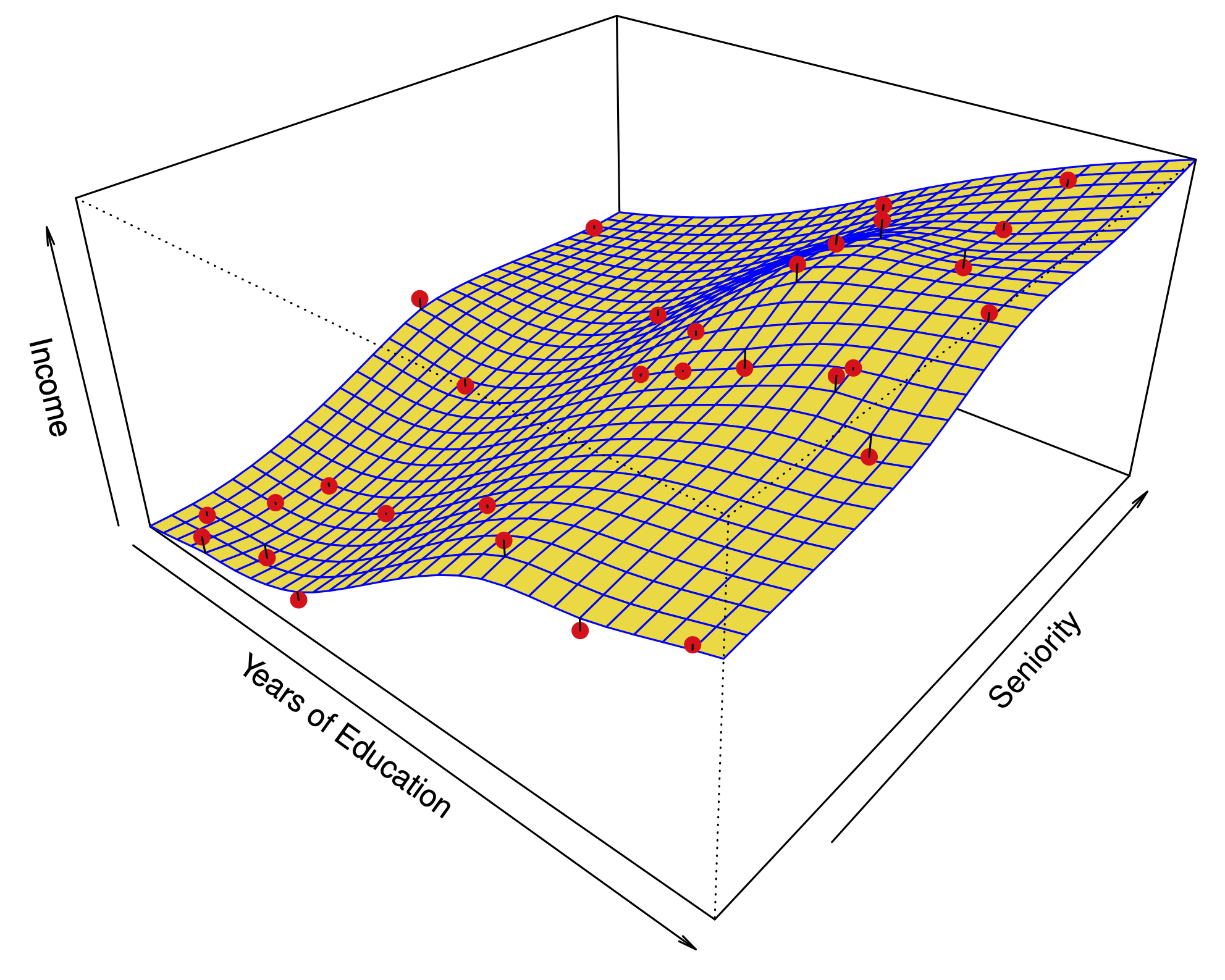
Visualizing the residuals can reveal phenomena that are not accounted for by the model; eg. synergies or interactions:
Potential issues in linear regression#
Interactions between predictors
Non-linear relationships
Correlation of error terms
Non-constant variance of error (heteroskedasticity)
Outliers
High leverage points
Collinearity
Interactions between predictors#
Linear regression has an additive assumption: $\(\mathtt{sales} = \beta_0 + \beta_1\times\mathtt{tv}+ \beta_2\times\mathtt{radio}+\varepsilon\)$
i.e. An increase of 100 USD dollars in TV ads causes a fixed increase of \(100 \beta_2\) USD in sales on average, regardless of how much you spend on radio ads.
Interactions between predictors#
If we visualize the residuals, we see they are not evenly scattered around the plane. This could be caused by an interaction.
Interactions between predictors#
One way to deal with this is to include multiplicative variables in the model:
The interaction variable
tv * radiois high when bothtvandradioare high.
Interactions between predictors#
R makes it easy to include interaction variables in the model:
summary(lm(sales ~ TV + radio + radio:TV, data=Advertising))
Non-linearities#

Example: Auto dataset.
A scatterplot between a predictor and the response may reveal a non-linear relationship.
Non-linearities#
Solution: include polynomial terms in the model.
Could use other functions besides polynomials…
Non-linearities#

In 2 or 3 dimensions, this is easy to visualize. What do we do when we have too many predictors?
Correlation of error terms#
We assumed that the errors for each sample are independent:
What if this breaks down?
The main effect is that this invalidates any assertions about Standard Errors, confidence intervals, and hypothesis tests…
Example: Suppose that by accident, we duplicate the data (we use each sample twice). Then, the standard errors would be artificially smaller by a factor of \(\sqrt{2}\).
Correlation of error terms#
When could this happen in real life:
Time series: Each sample corresponds to a different point in time. The errors for samples that are close in time are correlated.
Spatial data: Each sample corresponds to a different location in space.
Grouped data: Imagine a study on predicting height from weight at birth. If some of the subjects in the study are in the same family, their shared environment could make them deviate from \(f(x)\) in similar ways.
Correlation of error terms#

Simulations of time series with increasing correlations between \(\varepsilon_i\).
Non-constant variance of error (heteroskedasticity)#
The variance of the error depends on some characteristics of the input features.
To diagnose this, we can plot residuals vs. fitted values:

Non-constant variance of error (heteroskedasticity)#
If the trend in variance is relatively simple, we can transform the response using a logarithm, for example.
Outliers#

Outliers from a model are points with very high errors.
While they may not affect the fit, they might affect our assessment of model quality.
Outliers#
Possible solutions:
- If we believe an outlier is due to an error in data collection, we can remove it.
- An outlier might be evidence of a missing predictor, or the need to specify a more complex model.
High leverage points#

Some samples with extreme inputs have an outsized effect on \(\hat \beta\).
This can be measured with the leverage statistic or self influence:
Studentized residuals#
The residual \(e_i = y_i - \hat y_i\) is an estimate for the noise \(\epsilon_i\).
The standard error of \(\hat \epsilon_i\) is \(\sigma \sqrt{1-h_{ii}}\).
A studentized residual is \(\hat \epsilon_i\) divided by its standard error (with appropriate estimate of \(\sigma\))
When model is correct, it follows a Student-t distribution with \(n-p-2\) degrees of freedom.
Collinearity#

Two predictors are collinear if one explains the other well:
Collinearity#
*Problem: The coefficients become unidentifiable.
Consider the extreme case of using two identical predictors
limit: $\( \begin{aligned} \mathtt{balance} &= \beta_0 + \beta_1\times\mathtt{limit} + \beta_2\times\mathtt{limit} + \epsilon \\ & = \beta_0 + (\beta_1+100)\times\mathtt{limit} + (\beta_2-100)\times\mathtt{limit} + \epsilon \end{aligned} \)$For every \((\beta_0,\beta_1,\beta_2)\) the fit at \((\beta_0,\beta_1,\beta_2)\) is just as good as at \((\beta_0,\beta_1+100,\beta_2-100)\).
Collinearity#

Collinearity#
If 2 variables are collinear, we can easily diagnose this using their correlation.
A group of \(q\) variables is multilinear if these variables “contain less information” than \(q\) independent variables.
Pairwise correlations may not reveal multilinear variables.
The Variance Inflation Factor (VIF) measures how predictable it is given the other variables, a proxy for how necessary a variable is:
Above, \(R^2_{X_j|X_{-j}}\) is the \(R^2\) statistic for Multiple Linear regression of the predictor \(X_j\) onto the remaining predictors.
Comparison to \(K\)-nearest neighbors#
Linear regression: prototypical parametric method. Easy for inference.
KNN regression: prototypical nonparametric method. Inference less clear.
KNN estimator#
\(K\)-nearest neighbors#

\(K=1\) on left, \(K=9\) on right.
Comparing linear regression to \(K\)-nearest neighbors#
Linear regression: prototypical parametric method. Easy for inference.
KNN regression: prototypical nonparametric method. Inference less clear.
Long story short:#
KNN is only better when the function \(f\) is far from linear (in which case linear model is misspecified)
When \(n\) is not much larger than \(p\), even if \(f\) is nonlinear, Linear Regression can outperform KNN.
KNN has smaller bias, but this comes at a price of higher variance.
KNN estimates for a simulation from a linear model#

\(K=1\) on left, \(K=9\) on right.
Linear models dominate KNN#

Increasing deviations from linearity#

When there are more predictors than observations, Linear Regression dominates#

When \(p\gg n\), each sample has no near neighbors, this is known as the curse of dimensionality.
When there are more predictors than observations, Linear Regression dominates#
The variance of KNN regression is very large.