Best subset selection
Contents
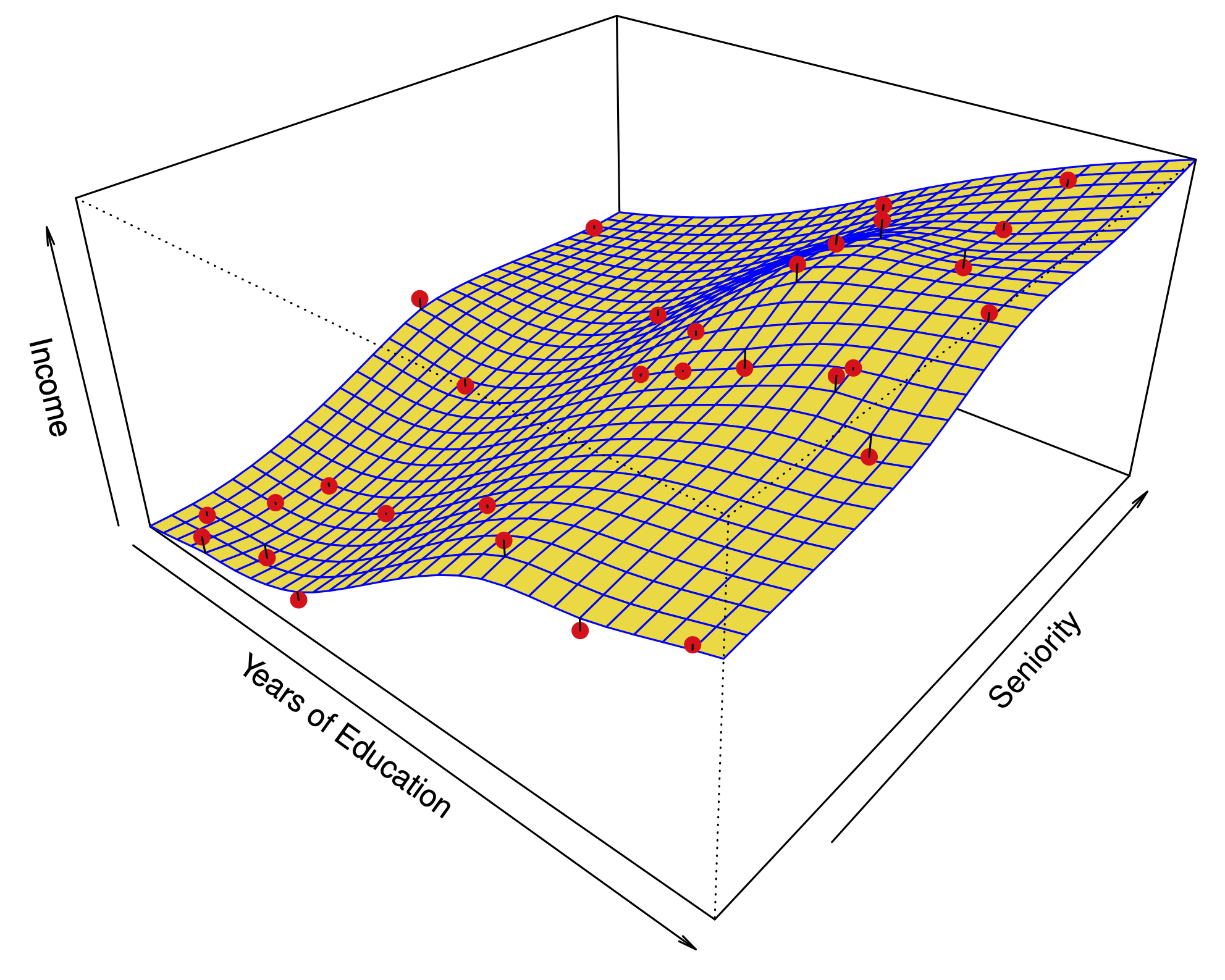
Let’s recap what we have learned about regression methods so far:
In linear regression, adding predictors always decreases the training error or RSS.
However, adding predictors does not necessarily improve the test error.
Selecting significant predictors is hard when \(n\) is not much larger than \(p\).
When \(n<p\), there is no least squares solution: $\(\hat \beta = \underbrace{(\mathbf{X}^T\mathbf{X})}_{\text{Singular}}^{-1}\mathbf{X}^T y.\)$
We should think about selecting fewer predictors.
Best subset selection#
Simple idea: let’s compare all models with \(k\) predictors.
There are \({p \choose k} = p!/\left[k!(p-k)!\right]\) possible models.
For every possible \(k\), choose the model with the smallest RSS.

Best subset with regsubsets#
library(ISLR) # where Credit is stored
library(leaps) # where regsubsets is found
summary(regsubsets(Balance ~ ., data=Credit))
Best model with 4 variables includes:
Cards, Income, Student, Limit.
Choosing \(k\)#
Naturally, \(\text{RSS}\) and $\( R^2 = 1-\frac{\text{RSS}}{\text{TSS}} \)\( improve as we increase \)k$.
To optimize \(k\), we want to minimize the test error, not the training error.
We could use cross-validation, or alternative estimates of test error:
Akaike Information Criterion (AIC) (closely related to Mallow’s \(C_p\)) given an estimate of the irreducible error \(\hat{\sigma^2}\) :
Bayesian Information Criterion (BIC):
Adjusted \(R^2\):
How do they compare to cross validation:
They are much less expensive to compute.
They are motivated by asymptotic arguments and rely on model assumptions (eg. normality of the errors).
Equivalent concepts for other models (e.g. logistic regression).
Example: best subset selection for the Credit dataset#

Best subset selection for the Credit dataset#

Recall: In \(K\)-fold cross validation, we can estimate a standard error or accuracy for our test error estimate. Then, we can apply the 1SE rule.
Stepwise selection methods#
Best subset selection has 2 problems:
It is often very expensive computationally. We have to fit \(2^p\) models!
If for a fixed \(k\), there are too many possibilities, we increase our chances of overfitting. The model selected has high variance.
In order to mitigate these problems, we can restrict our search space for the best model. This reduces the variance of the selected model at the expense of an increase in bias.
Forward selection#
- Let ${\cal M}_0$ denote the *null* model, which contains no predictors.
- For $k=0, \dots, p-1$:
- Consider all $p-k$ models that augment the predictors in ${\cal M}_k$ with one additional predictor.
- Choose the best among these $p-k$ models, and call it ${\cal M}_{k+1}$. Here *best* is defined as having smallest RSS or $R^2$.
- Select a single best model from among ${\cal M}_0, \dots, {\cal M}_p$ using cross-validated prediction error, AIC, BIC or adjusted $R^2$.
Forward selection in using step#
M.full = lm(Balance ~ ., data=Credit)
M.null = lm(Balance ~ 1, data=Credit)
step(M.null, scope=list(upper=M.full), direction='forward', trace=0)
First four variables are
Rating, Income, Student, Limit.Different from best subsets of size 4.
Backward selection#
- Let ${\cal M}_p$ denote the *full* model, which contains all $p$ predictors
- For $k=p,p-1,\dots,1$:
- Consider all $k$ models that contain all but one of the predictors in ${\cal M}_k$ for a total of $k-1$ predictors.
- Choose the best among these $k$ models, and call it ${\cal M}_{k-1}$. Here *best* is defined as having smallest RSS or $R^2$.
- Select a single best model from among ${\cal M}_0, \dots, {\cal M}_p$ using cross-validated prediction error, AIC, BIC or adjusted $R^2$.
Backward selection#
step(M.full, scope=list(lower=M.null), direction='backward', trace=0)
Forward selection with BIC#
step(M.null, scope=list(upper=M.full), direction='forward', trace=0, k=log(nrow(Credit))) # k defaults to 2, i.e AIC
Forward vs. backward selection#
- You cannot apply backward selection when $p>n$.
- Although we might like them to, they need not produce the same sequence of models.
- **Example:** $X_1,X_2 \sim \mathcal{N}(0,\sigma)$ independent and set $$ \begin{aligned} X_3 &= X_1 + 3 X_2 \\ Y &= X_1 + 2X_2 + \epsilon \end{aligned} $$
- Regress $Y$ onto $X_1,X_2,X_3$.
- Forward: $\{X_3\} \to \mathbf{\{X_3,X_2\} \text{or} \{X_3,X_1\}} \to \{X_3,X_2,X_1\}$
- Backward: $\{X_1,X_2,X_3\} \to \mathbf{ \{X_1,X_2\}} \to \{X_2\}$
Forward vs. backward selection#
n = 5000
X1 = rnorm(n)
X2 = rnorm(n)
X3 = X1 + 3 * X2
Y = X1 + 2 * X2 + rnorm(n)
D = data.frame(X1, X2, X3, Y)
Forward#
step(lm(Y ~ 1, data=D), list(upper=~ X1 + X2 + X3), direction='forward')
Backward#
step(lm(Y ~ X1 + X2 + X3, data=D), list(lower=~ 1), direction='backward')
Other stepwise selection strategies#
Mixed stepwise selection (
direction='both'): Do forward selection, but at every step, remove any variables that are no longer necessary.Forward stagewise selection: Roughly speaking, don’t add in the variable fully at each step…
\(\dots\)
Shrinkage methods#
A mainstay of modern statistics!
The idea is to perform a linear regression, while regularizing or shrinking the coefficients \(\hat \beta\) toward 0.
Why would shrunk coefficients be better?#
This introduces bias, but may significantly decrease the variance of the estimates. If the latter effect is larger, this would decrease the test error.
Extreme example: set \(\hat{\beta}\) to 0 – variance is 0!
There are Bayesian motivations to do this: priors concentrated near 0 tend to shrink the parameters’ posterior distribution.
Ridge regression#
Ridge regression solves the following optimization:
The RSS of the model at \(\beta\).
The squared \(\ell_2\) norm of \(\beta\), or \(\|\beta\|_2^2.\)
The parameter \(\lambda\) is a tuning parameter. It modulates the importance of fit vs. shrinkage.
We find an estimate \(\hat\beta^R_\lambda\) for many values of \(\lambda\) and then choose it by cross-validation. Fortunately, this is no more expensive than running a least-squares regression.
Ridge regression#
- In least-squares linear regression, scaling the variables has no effect on the fit of the model: $$Y = X_0 + \beta_1 X_1 + \beta_2 X_2 + \dots + \beta_p X_p.$$
- Multiplying $X_1$ by $c$ can be compensated by dividing $\hat \beta_1$ by $c$: after scaling we have the same RSS.
- In ridge regression, this is not true.
- In practice, what do we do?
- Scale each variable such that it has sample variance 1 before running the regression.
- This prevents penalizing some coefficients more than others.
Ridge regression of default in the Default dataset#

Ridge regression#

In a simulation study, we compute squared bias, variance, and test error as a function of \(\lambda\).
In practice, cross validation would yield an estimate of the test error but bias and variance are unobservable.
Selecting \(\lambda\) by cross-validation for ridge regression#

Lasso regression#
Lasso regression solves the following optimization:
RSS of the model at \(\beta\).
\(\ell_1\) norm of \(\beta\), or \(\|\beta\|_1.\)
The parameter \(\lambda\) is a tuning parameter. It modulates the importance of fit vs. shrinkage.
Why would we use the Lasso instead of Ridge regression?#
Ridge regression shrinks all the coefficients to a non-zero value.
The Lasso shrinks some of the coefficients all the way to zero.
A convex alternative (relaxation) to best subset selection (and its approximation stepwise selection)!
Ridge regression of default in the Default dataset#
A lot of pesky small coefficients throughout the regularization path
Lasso regression of default in the Default dataset#

Those coefficients are shrunk to zero
An alternative formulation for regularization#
- **Ridge:** for every $\lambda$, there is an $s$ such that $\hat \beta^R_\lambda$ solves:
$$\underset{\beta}{\text{minimize}} ~~\left\{\sum_{i=1}^n \left(y_i -\beta_0 -\sum_{j=1}^p \beta_j x_{i,j}\right)^2 \right\} ~~~ \text{subject to}~~~ \sum_{j=1}^p \beta_j^2
Visualizing Ridge and the Lasso with 2 predictors#

\(\color{BlueGreen}{\vardiamond}: ~\sum_{j=1}^p |\beta_j|<s ~~~~~~~~~~~~~~~~~~~~ \color{BlueGreen}{\CIRCLE}:~ \sum_{j=1}^p \beta_j^2<s~~~~~\), Best subset with \(s=1\) is union of the axes…
When is the Lasso better than Ridge?#

- **Example 1:** Most of the coefficients are non-zero.
- Bias, variance, MSE
- The Lasso (---), Ridge ($\cdots$).
- The bias is about the same for both methods.
- The variance of Ridge regression is smaller, so is the MSE.
When is the Lasso better than Ridge?#

- **Example 2:** Only 2 coefficients are non-zero.
- Bias, variance, MSE
- The Lasso (---), Ridge ($\cdots$).
- The bias, variance, and MSE are lower for the Lasso.
Selecting \(\lambda\) by cross-validation for lasso regression#

A very special case: ridge#
Suppose \(n=p\) and our matrix of predictors is \(\mathbf{X} = I\)
Then, the objective function in Ridge regression can be simplified: $\(\sum_{j=1}^p (y_j-\beta_j)^2 + \lambda\sum_{j=1}^p \beta_j^2\)$
We can minimize the terms that involve each \(\beta_j\) separately:
It is easy to show that
A very special case: LASSO#
Similar story for the Lasso; the objective function is:
We can minimize the terms that involve each \(\beta_j\) separately: $\((y_j-\beta_j)^2 + \lambda |\beta_j|.\)$
It is easy to show that $\(\hat \beta^L_j = \begin{cases} y_j -\lambda/2 & \text{if }y_j>\lambda/2; \\ y_j +\lambda/2 & \text{if }y_j<-\lambda/2; \\ 0 & \text{if }|y_j|<\lambda/2. \end{cases} \)$
Lasso and Ridge coefficients as a function of \(y\)#

Bayesian interpretation#

Ridge: \(\hat\beta^R\) is the posterior mean, with a Normal prior on \(\beta\).
Lasso: \(\hat\beta^L\) is the posterior mode, with a Laplace prior on \(\beta\).
Dimensionality reduction#
Regularization methods#
- Variable selection:
- Best subset selection
- Forward and backward stepwise selection
- Shrinkage
- Ridge regression
- The Lasso (a form of variable selection)
- Dimensionality reduction:
- **Idea:** Define a small set of $M$ predictors which *summarize* the information in all $p$ predictors.
Principal Component Regression#
Recall: The loadings \(\phi_{11}, \dots, \phi_{p1}\) for the first principal component define the directions of greatest variance in the space of variables.
princomp(USArrests, cor=TRUE)$loadings[,1] # cor=TRUE makes sure to scale variables
Interpretation: The first principal component measures the overall rate of crime.
Principal Component Regression#
Recall: The scores \(z_{11}, \dots, z_{n1}\) for the first principal component define the deviation of the samples along this direction.
princomp(USArrests, cor=TRUE)$scores[,1] # cor=TRUE makes sure to scale variables
Interpretation: The scores for the first principal component measure the overall rate of crime in each state.
Principal Component Regression#
- **Idea:**
- Replace the original predictors, $X_1, X_2, \dots, X_p$, with the first $M$ score vectors $Z_1, Z_2, \dots, Z_M$.
- Perform least squares regression, to obtain coefficients $\theta_0,\theta_1,\dots,\theta_M$.
- The model with these derived features is: $$ \begin{aligned} y_i &= \theta_0 + \theta_1 z_{i1} + \theta_2 z_{i2} + \dots + \theta_M z_{iM} + \varepsilon_i\\ & = \theta_0 + \theta_1 \sum_{j=1}^p \phi_{j1} x_{ij} + \theta_2 \sum_{j=1}^p \phi_{j2} x_{ij} + \dots + \theta_M \sum_{j=1}^p \phi_{jM} x_{ij} + \varepsilon_i \\ & = \theta_0 + \left[\sum_{m=1}^M \theta_m \phi_{1m}\right] x_{i1} + \dots + \left[\sum_{m=1}^M \theta_m \phi_{pm}\right] x_{ip} + \varepsilon_i \end{aligned} $$
- Equivalent to a linear regression onto $X_1,\dots,X_p$, with coefficients: $$\beta_j = \sum_{m=1}^M \theta_m \phi_{jm}$$
- This constraint in the form of $\beta_j$ introduces *bias*, but it can lower the *variance* of the model.
Application to the Credit dataset#

A model with 11 components is equivalent to least-squares regression
Best CV error is achieved with 10 components (almost no dimensionality reduction)
Application to the Credit dataset#
The left panel shows the coefficients \(\beta_j\) estimated for each \(M\).
The coefficients shrink as we decrease \(M\)!
Relationship between PCR and Ridge regression#
- **Least squares regression:** want to minimize $$RSS = (y-\mathbf{X}\beta)^T(y-\mathbf{X}\beta)$$
- **Score equation:** $$\frac{\partial RSS}{\partial \beta} = -2\mathbf{X}^T(y-\mathbf{X}\beta) = 0$$
- **Solution:** $$\implies \hat \beta = (\mathbf{X}^T\mathbf{X})^{-1}\mathbf{X}^T y$$
- Compute singular value decomposition: $\mathbf{X} = U D^{1/2} V^T$, where $D^{1/2} = \text{diag}(\sqrt{d_1},\dots,\sqrt{d_p})$.
- Then $$(\mathbf{X}^T\mathbf{X})^{-1} = V D^{-1} V^T$$ where $D^{-1} = \text{diag}(1/d_1,1/d_2,\dots,1/d_p)$.
Relationship between PCR and Ridge regression#
- **Ridge regression:** want to minimize $$RSS + \lambda \|\beta\|_2^2 = (y-\mathbf{X}\beta)^T(y-\mathbf{X}\beta) + \lambda \beta^T\beta$$ $$RSS = (y-\mathbf{X}\beta)^T(y-\mathbf{X}\beta)$$
- **Score equation:** $$\frac{\partial (RSS + \lambda \|\beta\|_2^2)}{\partial \beta} = -2\mathbf{X}^T(y-\mathbf{X}\beta) + 2\lambda\beta= 0$$
- **Solution:** $$\implies \hat \beta^R_\lambda = (\mathbf{X}^T\mathbf{X} + \lambda I)^{-1}\mathbf{X}^T y$$
- Note $$(\mathbf{X}^T\mathbf{X}+ \lambda I)^{-1} = V D_\lambda ^{-1} V^T$$ where $D_\lambda ^{-1} = \text{diag}(1/(d_1+\lambda),1/(d_2+\lambda),\dots,1/(d_p+\lambda))$.
Relationship between PCR and Ridge regression#
- **Predictions of least squares regression:** $$\hat y = \mathbf{X}\hat \beta = \sum_{j=1}^p u_j u_j^T y, \qquad u_j \text{ is the } j\text{th column of } U$$
- **Predictions of Ridge regression:** $$\hat y = \mathbf{X}\hat \beta^R_\lambda = \sum_{j=1}^p u_j \frac{d_j}{d_j + \lambda} u_j^T y$$ The projection of $y$ onto a principal component is shrunk toward zero. The smaller the principal component, the larger the shrinkage.
- **Predictions of PCR:** $$\hat y = \mathbf{X}\hat \beta^\text{PC} = \sum_{j=1}^p u_j \mathbf{1}(j\leq M) u_j^T y$$ The projections onto small principal components are shrunk to zero.
Principal Component Regression#

- In each case $n=50$, $p=45$.
- Left: response is a function of all the predictors (*dense*).
- Right: response is a function of 2 predictors (*sparse* - good for Lasso).
Principal Component Regression#
Ridge and Lasso on dense dataset
The Lasso (—), Ridge (\(\cdots\)).
PCR seems at least comparable to optimal LASSO and ridge.
Principal Component Regression#
Ridge and Lasso on sparse dataset
The Lasso (—), Ridge (\(\cdots\)).
Lasso clearly better than PCR here.
Principal Component Regression#

- Again, $n=50$, $p=45$.
- The response is a function of the first 5 principal components.
Partial least squares#
Principal components regression derives \(Z_1,\dots,Z_M\) using only the predictors \(X_1,\dots,X_p\).
In partial least squares, we use the response \(Y\) as well. (To be fair, best subsets and stepwise do as well.)
Algorithm:#
- Define $Z_1 = \sum_{j=1}^p \phi_{j1} X_j$, where $\phi_{j1}$ is the coefficient of a simple linear regression of $Y$ onto $X_j$.
- Let $X_j^{(2)}$ be the residual of regressing $X_j$ onto $Z_1$.
- Define $Z_2 = \sum_{j=1}^p \phi_{j2} X_j^{(2)}$, where $\phi_{j2}$ is the coefficient of a simple linear regression of $Y$ onto $X_j^{(2)}$.
- Let $X_j^{(3)}$ be the residual of regressing $X_j^{(2)}$ onto $Z_2$.
- ...
Partial least squares#
- At each step, we try to find the linear combination of predictors that is highly correlated to the response (the highest correlation is the least squares fit).
- After each step, we transform the predictors such that they are \emph{uncorrelated} from the linear combination chosen.
- Compared to PCR, partial least squares has less bias and more variance (a stronger tendency to overfit).
High-dimensional regression#
- Most of the methods we've discussed work best when $n$ is much larger than $p$.
- However, the case $p\gg n$ is now common, due to experimental advances and cheaper computers:
- **Medicine:** Instead of regressing heart disease onto just a few clinical observations (blood pressure, salt consumption, age), we use in addition 500,000 single nucleotide polymorphisms.
- **Marketing:** Using search terms to understand online shopping patterns. A \emph{bag of words} model defines one feature for every possible search term, which counts the number of times the term appears in a person's search. There can be as many features as words in the dictionary.
Some problems#

When \(n=p\), we can find a fit that goes through every point.
We could use regularization methods, such as variable selection, ridge regression and the lasso.
Some problems#

Measures of training error are really bad.
Furthermore, it becomes hard to estimate the noise \(\hat \sigma^2\).
Measures of model fit \(C_p\), AIC, and BIC fail.
Some problems#

In each case, only 20 predictors are associated to the response.
Plots show the test error of the Lasso.
Message: Adding predictors that are uncorrelated with the response hurts the performance of the regression!
Interpreting coefficients when \(p>n\)#
When \(p>n\), every predictor is a linear combination of other predictors, i.e.\ there is an extreme level of multicollinearity.
The Lasso and Ridge regression will choose one set of coefficients.
The coefficients selected \(\{i\;;\; |\hat\beta_i| >\delta \}\) are not guaranteed to be identical to \(\{i\;;\; |\beta_i| >\delta \}\). There can be many sets of predictors (possibly non-overlapping) which yield apparently good models.
Message: Don’t overstate the importance of the predictors selected.
Interpreting inference when \(p>n\)#
When \(p>n\), LASSO might select a sparse model.
Running
lmon selected variables on training data is bad.Running
lmon selected variables on independent validation data is OK-ish – is thislma good model?Message: Don’t use inferential methods developed for least squares regression for things like LASSO, forward stepwise, etc.
Can we do better? Yes, but it’s complicated and a little above our level here.