Non-linear regression
Contents
Non-linear regression#

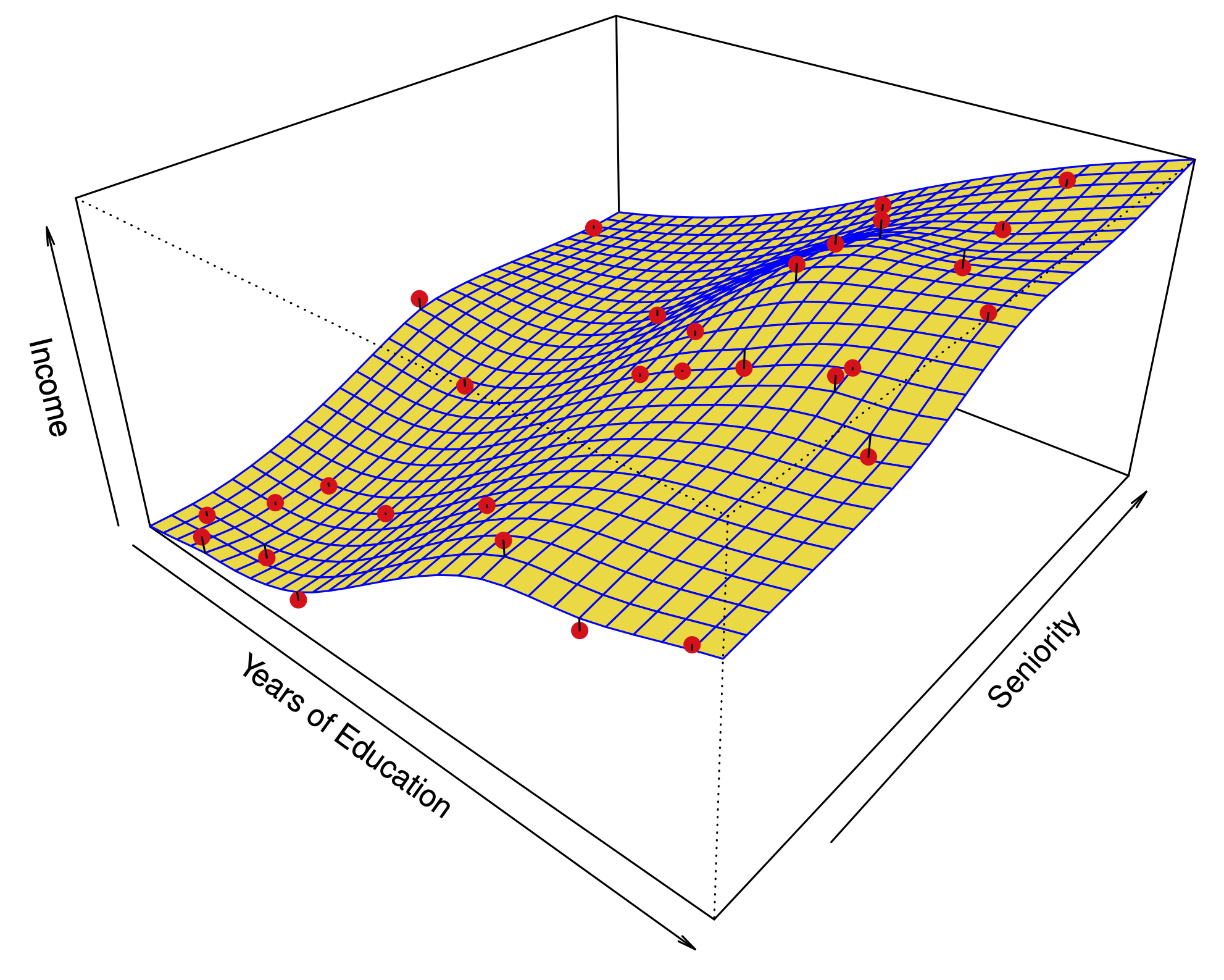
Problem: How do we model a non-linear relationship?
Left: Regression of
wageontoage.Right: Logistic regression for classes
wage>250andwage<250
Basis functions#
Strategy:
- Define a model: $$Y = \beta_0 + \beta_1 f_1(X) + \beta_2 f_2(X) + \dots + \beta_d f_d(X) + \epsilon.$$
- Fit this model through least-squares regression: $f_j$'s are nonlinear, model is linear!
- Some options for $f_1,\dots,f_d$:
- Polynomials, $f_i(x) = x^i$.
- Indicator functions, $f_i(x) = \mathbf{1}(c_i \leq x < c_{i+1})$.
Piecewise constant#

Piecewise polynomials#

Cubic splines#
- Define a set of knots $\xi_1< \xi_2 < \dots<\xi_K$.
- We want the function $f$ in $Y= f(X) + \epsilon$ to:
- Be a cubic polynomial between every pair of knots $\xi_i,\xi_{i+1}$.
- Be continuous at each knot.
- Have continuous first and second derivatives at each knot.
- It turns out, we can write $f$ in terms of $K+3$ basis functions: $$f(X) = \beta_0 + \beta_1 X + \beta_2 X^2 + \beta_3 X^3 + \beta_4 h(X,\xi_1) + \dots + \beta_{K+3} h(X,\xi_K)$$
- Above, $$ h(x,\xi) = \begin{cases} (x-\xi)^3 \quad \text{if }x>\xi \\ 0 \quad \text{otherwise} \end{cases} $$
Natural cubic splines#

Spline which is linear instead of cubic for \(X<\xi_1\), \(X>\xi_K\).
The predictions are more stable for extreme values of \(X\).
Choosing the number and locations of knots#

The locations of the knots are typically quantiles of \(X\).
The number of knots, \(K\), is chosen by cross validation:
Natural cubic splines vs. polynomial regression#

Splines can fit complex functions with few parameters.
Polynomials require high degree terms to be flexible.
High-degree polynomials can be unstable at the edges.
Smoothing splines#
Find the function \(f\) which minimizes
The RSS when using \(f\) to predict.
A penalty for the roughness of the function.
Facts#
The minimizer \(\hat f\) is a natural cubic spline, with knots at each sample point \(x_1,\dots,x_n\).
Obtaining \(\hat f\) is similar to a Ridge regression.
Advanced: deriving a smoothing spline#
- Show that if you fix the values $f(x_1),\dots,f(x_2)$, the roughness $$\int f''(x)^2 dx$$ is minimized by a natural cubic spline.
- Deduce that the solution to the smoothing spline problem is a natural cubic spline, which can be written in terms of its basis functions. $$f(x) = \beta_0 + \beta_1 f_1(x) + \dots \beta_{n+3} f_{n+3}(x)$$
- Letting $\mathbf N$ be a matrix with $\mathbf N(i,j) = f_j(x_i)$, we can write the objective function: $$ (y - \mathbf N\beta)^T(y - \mathbf N\beta) + \lambda \beta^T \Omega_{\mathbf N}\beta, $$ where $\Omega_{\mathbf N}(i,j) = \int N_i''(t) N_j''(t) dt$.
Advanced: deriving a smoothing spline#
- By simple calculus, the coefficients $\hat \beta$ which minimize $$ (y - \mathbf N\beta)^T(y - \mathbf N\beta) + \lambda \beta^T \Omega_{\mathbf N}\beta, $$ are $\hat \beta = (\mathbf N^T \mathbf N + \lambda \Omega_{\mathbf N})^{-1} \mathbf N^T y$.
- Note that the predicted values are a linear function of the observed values: $$\hat y = \underbrace{\mathbf N (\mathbf N^T \mathbf N + \lambda \Omega_{\mathbf N})^{-1} \mathbf N^T}_{\mathbf S_\lambda} y$$
- The **degrees of freedom** for a smoothing spline are: $$\text{Trace}(\mathbf S_\lambda)= \mathbf S_\lambda(1,1) + \mathbf S_\lambda(2,2) + \cdots + \mathbf S_\lambda(n,n) $$
Natural cubic splines vs. Smoothing splines#
| **Natural cubic splines** | **Smoothing splines** |
|
|
Choosing the regularization parameter \(\lambda\)#
We typically choose \(\lambda\) through cross validation.
Fortunately, we can solve the problem for any \(\lambda\) with the same complexity of diagonalizing an \(n\times n\) matrix.
There is a shortcut for LOOCV: $\( \begin{aligned} RSS_\text{loocv}(\lambda) &= \sum_{i=1}^n (y_i - \hat f_\lambda^{(-i)}(x_i))^2 \\ &= \sum_{i=1}^n \left[\frac{y_i-\hat f_\lambda(x_i)}{1-\mathbf S_\lambda(i,i)}\right]^2 \end{aligned} \)$
Choosing the regularization parameter \(\lambda\)#

Local linear regression#

Sample points nearer \(x\) are weighted higher in corresponding regression.
Algorithm#
To predict the regression function \(f\) at an input \(x\):
- Assign a weight $K_i(x)$ to the training point $x_i$, such that:
- $K_i(x)=0$ unless $x_i$ is one of the $k$ nearest neighbors of $x$ (not strictly necessary).
- $K_i(x)$ decreases when the distance $d(x,x_i)$ increases.
- Perform a **weighted least squares** regression; i.e. find $(\beta_0,\beta_1)$ which minimize $$\hat{\beta}(x) = \text{argmin}_{(\beta_0, \beta_1)} \sum_{i=i}^n K_i(x) (y_i - \beta_0 -\beta_1 x_i)^2.$$
- Predict $\hat f(x) = \hat \beta_0(x) + \hat \beta_1(x) x$.
Generalized nearest neighbors#
- Set $K_i(x)=1$ if $x_i$ is one of $x$'s $k$ nearest neighbors.
- Perform a ``regression'' with only an intercept; i.e. find $\beta_0$ which minimizes $$\hat{\beta}_0(x) = \text{argmin}_{\beta_0} \sum_{i=i}^n K_i(x)(y_i - \beta_0)^2.$$
- Predict $\hat f(x) = \hat \beta_0(x)$.
- Common choice that is smoother than nearest neighbors $$K_i(x) = \exp(-\|x-x_i\|^2/2\lambda)$$
Local linear regression#

The span \(k/n\), is chosen by cross-validation.
Generalized Additive Models (GAMs)#
Extension of non-linear models to multiple predictors:
The functions \(f_1,\dots,f_p\) can be polynomials, natural splines, smoothing splines, local regressions…
Fitting a GAM#
- If the functions $f_1$ have a basis representation, we can simply use least squares:
- Natural cubic splines
- Polynomials
- Step functions
Fitting a GAM#
- Otherwise, we can use **backfitting**:
- Keep $\beta_0,f_2,\dots,f_p$ fixed, and fit $f_1$ using the partial residuals: $$y_i - \beta_0 - f_2( x_{i2}) -\dots - f_p( x_{ip}),$$ as the response.
- Keep $\beta_0,f_1,f_3,\dots,f_p$ fixed, and fit $f_2$ using the partial residuals: $$y_i - \beta_0 - f_1( x_{i1}) - f_3( x_{i3}) -\dots - f_p( x_{ip}),$$ as the response.
- ...
- Iterate
- This works for smoothing splines and local regression.
- **For smoothing splines this is a descent method, descending on convex loss ...**
Backfitting: coordinate descent#
- Also works for linear regression...
- Initialize $\hat{\beta}^{(0)} = 0$ and, (say).
- Given $\hat{\beta}^{(T-1)}$, choose a coordinate $0 \leq k(T) \leq p$ and find $$ \begin{aligned} \hat{\alpha}(T) &= \text{argmin}_{\alpha} \sum_{i=1}^n\left(Y_i - \hat{\beta}^{(T-1)}_0 - \sum_{j:j \neq k(T)} X_{ij} \hat{\beta}^{(T-1)}_j - \alpha X_{ik(T)}\right)^2 \\ &= \frac{\sum_{i=1}^n X_{ik(T)}\left(Y_i - \hat{\beta}^{(T-1)}_0 - \sum_{j: j \neq k(T)} X_{ij} \hat{\beta}^{(T-1)}_j\right)} {\sum_{i=1}^n X_{ik(T)}^2} \end{aligned} $$
- Set $\hat{\beta}^{(T)}=\hat{\beta}^{(T-1)}$ except $k(T)$ entry which we set to $\hat{\alpha}(T)$.
- Iterate
Backfitting: coordinate descent and LASSO#
- Also works for LASSO...
- Initialize $\hat{\beta}^{(0)} = 0$ and, (say).
- Given $\hat{\beta}^{(T-1)}$, choose a coordinate $0 \leq k(T) \leq p$ and find $$ \begin{aligned} \hat{\alpha}_{\lambda}(T) &= \text{argmin}_{\alpha} \sum_{i=1}^n\left(r^{(T-1)}_{ik(T)} - \alpha X_{ik(T)}\right)^2 \\ & \qquad + \lambda \sum_{j: j \neq k(T)} |\hat{\beta}^{(T-1)}_j| + \lambda |\alpha| \end{aligned} $$ with $r^{(T-1)}_j$ the $j$-th partial residual at iteration $T$ $$ r^{(T-1)}_j = Y - \hat{\beta}^{(T-1)}_0 - \sum_{l:l \neq j} X_l \hat{\beta}^{(T-1)}_l. $$ Solution is a simple soft-thresholded version of previous $\hat{\alpha}(T)$ -- **Very fast! Used in `glmnet`**
- Set $\hat{\beta}^{(T)}=\hat{\beta}^{(T-1)}$ except $k(T)$ entry which we set to $\hat{\alpha}_{\lambda}(T)$.
- Iterate...
Backfitting: GAM#
- Let's look at basis functions
- Initialize $\hat{\beta}^{(0)} = 0$ and, (say).
- Given $\hat{\beta}^{(T-1)}$, choose a coordinate $0 \leq k(T) \leq p$ and find $$ \begin{aligned} \hat{\alpha}(T) &= \text{argmin}_{\alpha \in \mathbb{R}^{n_{k(T)}}} \\ & \qquad \sum_{i=1}^n\biggl(Y_i - \hat{\beta}^{(T-1)}_0 - \sum_{j:j \neq k(T)} \sum_{l=1}^{n_j} f_{lj}(X_{ij}) \hat{\beta}^{(T-1)}_{lj} \\ & \qquad \quad - \sum_{l=1}^{n_{k(T)}} \alpha_{l} f_{lk(T)}(X_{ik(T)})\biggr)^2 \end{aligned} $$
- Set $\hat{\beta}^{(T)}=\hat{\beta}^{(T-1)}$ except $k(T)$ entries which we set to $\hat{\alpha}(T)$. **Blockwise coordinate descent!**
- Iterate...
Properties#
- GAMs are a step from linear regression toward a fully nonparametric method.
- The only constraint is additivity. This can be partially addressed by adding key interaction variables $X_iX_j$ (or tensor product of basis functions -- e.g. polynomials of two variables).
- We can report degrees of freedom for many non-linear functions.
- As in linear regression, we can examine the significance of each of the variables.
Example: Regression for Wage#

year: natural spline with df=4.age: natural spline with df=5.education: factor.
Example: Regression for Wage#

year: smoothing spline with df=4.age: smoothing spline with df=5.education: step function
Classification#
We can model the log-odds in a classification problem using a GAM:
Again fit by backfitting …
Backfitting: GAM with logistic loss#
- Also works for logistic...
- Initialize $\hat{\beta}^{(0)} = 0$ and, (say).
- Given $\hat{\beta}^{(T-1)}$, choose a coordinate $0 \leq k(T) \leq p$ with $\ell$ logistic loss, find $$ \begin{aligned} \hat{\alpha}(T) &= \text{argmin}_{\alpha \in \mathbb{R}^{n_{k(T)}}} \\ & \qquad \sum_{i=1}^n \ell\biggl(Y_i, \hat{\beta}^{(T-1)}_0 + \sum_{j:j \neq k(T)} \sum_{l=1}^{n_j} f_{lj}(X_{ij}) \hat{\beta}^{(T-1)}_{lj} \\ & \qquad \quad + \sum_{l=1}^{n_{k(T)}} \alpha_{l} f_{lk(T)}(X_{ik(T)}) \biggr) \end{aligned} $$
- Set $\hat{\beta}^{(T)}=\hat{\beta}^{(T-1)}$ except $k(T)$ entries which we set to $\hat{\alpha}(T)$.
- Works for losses that have a *linear predictor*.
- For GAMs, the linear predictor is $$ \beta_0 + f_1(X_1) + \dots + f_p(X_p) $$
Example: Classification for Wage>250#

year: linearage: smoothing spline with df=5education: step function
Example: Classification for Wage>250#

Same model excluding cases
education == "<HS"