Validation
Contents
Thinking about the true loss function is important
Most of the {\bf regression} methods we’ve studied aim to minimize the RSS, while {\bf classification} methods aim to minimize the 0-1 loss.
In classification, we often care about certain kinds of error more than others; i.e. the natural loss function is not the 0-1 loss.
Even if we use a method which minimizes a certain kind of training error, we can tune it to optimize our true loss function.
Example: in the
defaultstudy we could find the threshold that brings the False negative rate below an acceptable level.
Validation#
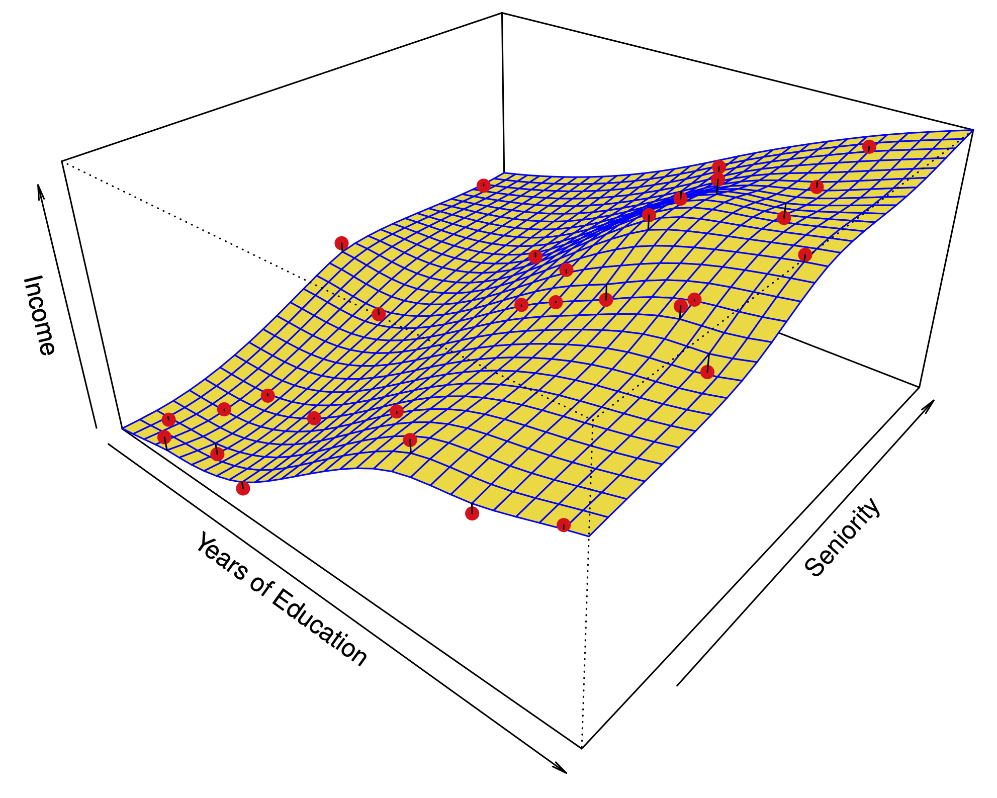
- **Problem:** Choose a supervised method that minimizes the test error.
- In addition, *tune* the parameters of each method: maybe
- $k$ in $k$-nearest neighbors.
- The number of variables to include in forward or backward selection.
- The order of a polynomial in polynomial regression.
Validation set approach#
Use of a validation set is one way to approximate the test error:
Divide the data into two parts.
Train each model with one part.
Compute the error on the remaining validation data.

Example: choosing order of polynomial#

Polynomial regression to estimate
mpgfromhorsepowerin the Auto data.Problem: Every split yields a different estimate of the error.
Leave one out cross-validation (LOOCV)#
- For every $i=1,\dots,n$:
- train the model on every point except $i$,
- compute the test error on the held out point.
- Average the test errors.
Regression#
Overall error: $\(\text{CV}_{(n)} = \frac{1}{n}\sum_{i=1}^n (y_i - \color{Red}{\hat y_i^{(-i)}})^2\)$
Notation \hat y_i^{(-i)}: prediction for the \(i\) sample when learning without using the \(i\)th sample.
Example: ?#

Algorithm 5.2?: LOOCV#
- For every $i=1,\dots,n$:
- train the model on every point except $i$,
- compute the test error on the held out point.
- Average the test errors.
Classification#
Overall error: $\(\text{CV}_{(n)} = \frac{1}{n}\sum_{i=1}^n \mathbf{1}(y_i \neq \color{Red}{\hat y_i^{(-i)}})\)$
Here, \hat y_i^{(-i)} is predicted label for the \(i\) sample when learning without using the \(i\)th sample.
Shortcut for linear regression#
Computing \(\text{CV}_{(n)}\) can be computationally expensive, since it involves fitting the model \(n\) times.
For linear regression, there is a shortcut:
Above, \(h_{ii}\) is the leverage statistic.
Approximate versions sometimes used for logistic regression…
\(K\)-fold cross-validation#
Algorithm 5.3? \(K\)-fold CV#
- Split the data into $K$ subsets or *folds*.
- For every $i=1,\dots,K$:
- train the model on every fold except the $i$th fold,
- compute the test error on the $i$th fold.
- Average the test errors.
Example: ?#

LOOCV vs. \(K\)-fold cross-validation#

\(K\)-fold CV depends on the chosen split (somewhat).
In \(K\)-fold CV, we train the model on less data than what is available. This introduces bias into the estimates of test error.
In LOOCV, the training samples highly resemble each other. This increases the variance of the test error estimate.
\(n\)-fold CV is equivalent LOOCV.
Choosing an optimal model#

Even if the error estimates are off, choosing the model with the minimum cross validation error often leads to a method with near minimum test error.

In a classification problem, things look similar.
– – – Bayes boundary,—— Logistic regression with polynomial predictors of increasing degree.
Choosing an optimal model#

In a classification problem, things look similar.
The one standard error (1SE) rule of thumb#

|
|
The wrong way to do cross validation#
- *Reading:* Section 7.10.2 of The Elements of Statistical Learning.
- We want to classify 200 individuals according to whether they have cancer or not.
- We use logistic regression onto 1000 measurements of gene expression.
- **Proposed strategy:**
- Using all the data, select the 20 most significant genes using $z$-tests.
- Estimate the test error of logistic regression with these 20 predictors via 10-fold cross validation.
The wrong way to do cross validation#
- To see how that works, let's use the following simulated data:
- Each gene expression is standard normal and independent of all others.
- The response (cancer or not) is sampled from a coin flip --- no correlation to any of the "genes".
- Q: What should the misclassification rate be for any classification method using these predictors?
- A: Roughly 50%.
The wrong way to do cross validation#
- We run this simulation, and obtain a CV error rate of 3%!
- Why?
- Since we only have 200 individuals in total, among 1000 variables, at least some will be correlated with the response.
- We had run variable selection using \emph{all the data}, so the variables we select have some correlation with the response in every subset or fold in the cross validation.
The right way to do cross validation#
- Divide the data into 10 folds.
- For $i=1,\dots,10$:
- Using every fold except $i$, perform the variable selection and fit the model with the selected variables.
- Compute the error on fold $i$.
- Average the 10 test errors obtained.
In our simulation, this produces an error estimate of close to 50%.
Moral of the story: Every aspect of the learning method that involves using the data — variable selection, for example — must be cross-validated.
Bootstrap#
Another resampling technique often seen in practice.
Cross-validation vs. the Bootstrap#
Cross-validation: provides estimates of the (test) error
The Bootstrap: provides the (standard) error of estimates
Bootstrap#

|
- One of the most important techniques in all of Statistics.
|
Standard errors in linear regression from a sample of size \(n\)#
summary(M.sales)
Classical way to compute Standard Errors#
- **Example:** Estimate the variance of a sample $x_1,x_2,\dots,x_n$:
- Unbiased estimate of $\sigma^2$: $$\hat \sigma^2 = \frac{1}{n-1}\sum_{i=1}^n (x_i-\overline x)^2.$$
- What is the Standard Error of $\hat \sigma^2$?
- Assume that $x_1,\dots,x_n$ are normally distributed with common mean $\mu$ and variance $\sigma^2$.
- Then $\hat \sigma^2(n-1)$ has a $\chi$-squared distribution with $n-1$ degrees of freedom.
- For large $n$, $\hat{\sigma}^2$ is normally distributed around $\sigma^2$.
- The SD of this *sampling distribution* is the Standard Error.
Limitations of the classical approach#
- This approach has served statisticians well for many years; however, what happens if:
- The distributional assumption --- for example, $x_1,\dots,x_n$ being normal --- breaks down?
- The estimator does not have a simple form and its sampling distribution cannot be derived analytically?
Example: Investing in two assets#

Suppose that \(X\) and \(Y\) are the returns of two assets.
These returns are observed every day: \((x_1,y_1),\dots,(x_n,y_n)\).
Example. Investing in two assets#
We have a fixed amount of money to invest and we will invest a fraction \(\alpha\) on \(X\) and a fraction \((1-\alpha)\) on \(Y\).
Therefore, our return will be
Our goal will be to minimize the variance of our return as a function of \(\alpha\).
One can show that the optimal \(\alpha\) is: $\(\alpha = \frac{\sigma_Y^2 - \text{Cov}(X,Y)}{\sigma_X^2 + \sigma_Y^2 -2\text{Cov}(X,Y)}.\)$
Proposal: Use an estimate: $\(\hat \alpha = \frac{\hat \sigma_Y^2 - \hat{ \text{Cov}}(X,Y)}{\hat \sigma_X^2 + \hat \sigma_Y^2 -2\hat{ \text{Cov}}(X,Y)}.\)$
Example: Investing in two assets#
Suppose we compute the estimate \(\hat\alpha = 0.6\) using the samples \((x_1,y_1),\dots,(x_n,y_n)\).
How sure can we be of this value? (A little vague of a question.)
If we had sampled the observations in a different 100 days, would we get a wildly different \(\hat \alpha\)? (A more precise question.) \ei
Resampling the data from the true distribution#

In this thought experiment, we know the actual joint distribution \(P(X,Y)\), so we can resample the \(n\) observations to our hearts’ content.
Computing the standard error of \(\hat \alpha\)#
We will use \(S\) samples to estimate the standard error of \(\hat{\alpha}\).
For each sampling of the data, for \(1 \leq s \leq S\)
we can compute a value of the estimate \(\hat \alpha^{(1)},\hat \alpha^{(2)},\dots\).
The Standard Error of \(\hat \alpha\) is approximated by the standard deviation of these values.
In reality, we only have \(n\) samples#
|
|
\[\hat P(X,Y) = \frac{1}{n}\sum_{i=1}^{n} \delta(x_i,y_i).\]
|
A schematic of the Bootstrap#

Comparing Bootstrap sampling to sampling from the true distribution#
