Principal Components Analysis
Contents
Principal Components Analysis#
Some facts#
This is the most popular unsupervised procedure ever.
Invented by Karl Pearson (1901).
Developed by Harold Hotelling (1933). \(\leftarrow\) Stanford pride!
What does it do? It provides a way to visualize high dimensional data, summarizing the most important information.
What is PCA good for?#
 |
 |
What is the first principal component?#
It is the vector which passes the closest to a cloud of samples, in terms of squared Euclidean distance.

Geometric interpretation#
i.e. The green direction minimizes the average squared length of the dotted lines.

What does this look like with 3 variables?#
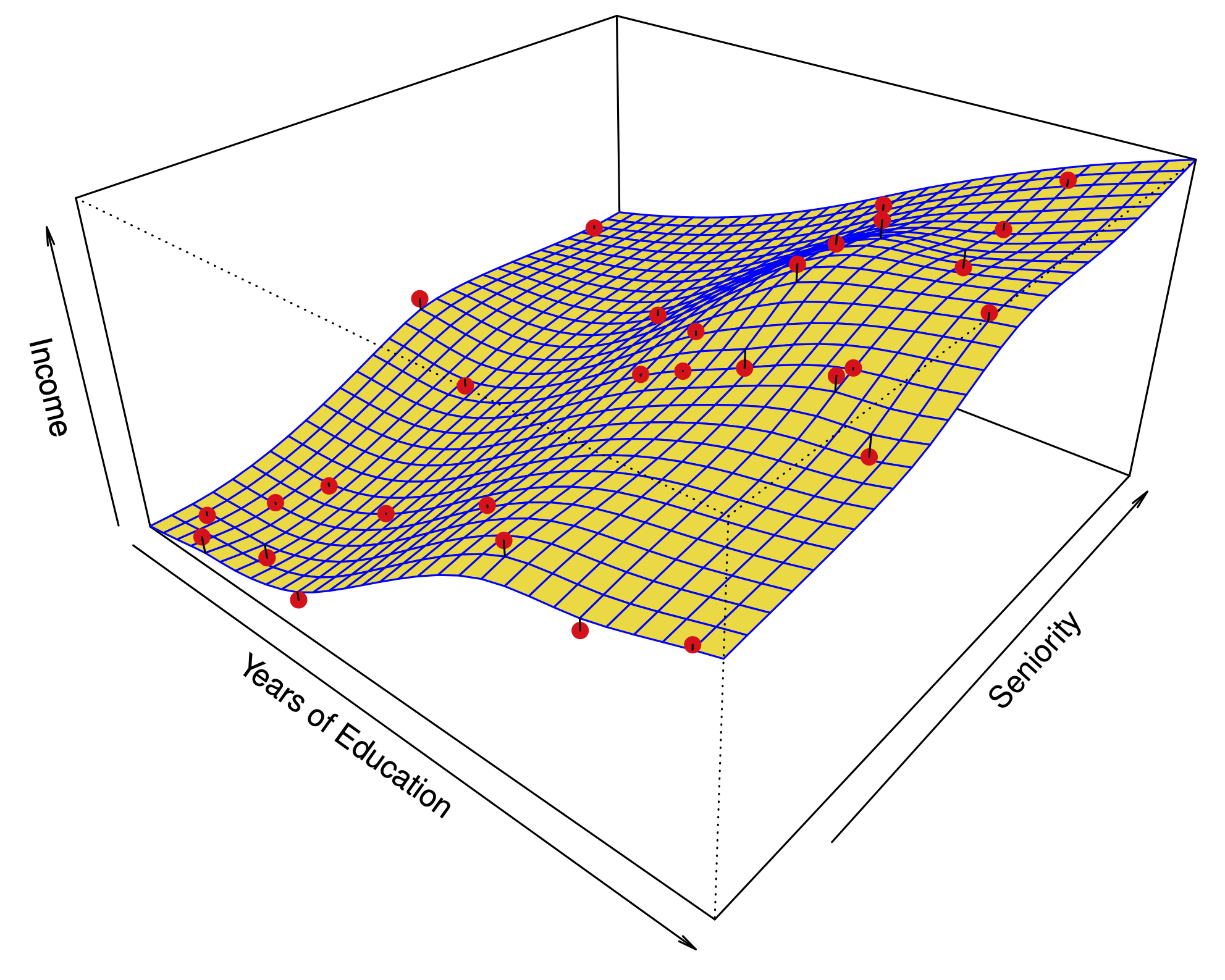
The first two principal components span a plane which is closest to the data.
 |
 |
A second interpretation#
The projection onto the first principal component is the one with the highest variance.
How do we say this in math?#
Let \(\mathbf{X}\) be a data matrix with \(n\) samples, and \(p\) variables.
From each variable, we subtract the mean of the column; i.e. we center the variables.
To find the first principal component \(\phi_1 = (\phi_{11},\dots,\phi_{p1})\), we solve the following optimization
The quantity $\( \sum_{j=1}^p x_{ij} \phi_{j1} = X\phi_1. \)$
Summing the square of the entries of \(Z\) computes the variance of the \(n\) samples projected onto \(\phi_1\). (This is a variance because we have centered the columns.)
Having found the maximizer \(\hat{\phi}_1\), the quantity $\( Z_1 = X\hat{\phi}_1 \)$ is the first principal component score.
How do we say this in math?#
To find the second principal component \(\phi_2 = (\phi_{12},\dots,\phi_{p2})\), we solve the following optimization $\( \begin{aligned} \max_{\phi_{12},\dots,\phi_{p2}} \left\{ \frac{1}{n}\sum_{i=1}^n \left( \sum_{j=1}^p \phi_{j2}x_{ij} \right)^2 \right\} \\ \text{ subject to} \;\;\sum_{j=1}^p \phi_{j2}^2 =1 \;\;\text{ and }\;\; \sum_{j=1}^p \hat{\phi}_{j1}\phi_{j2} = 0. \end{aligned} \)$
The second constraint \(\hat{\phi}_1^T\phi_2=0\) forces first and second principal components to be orthogonal.
Having found the optimal \(\hat{\phi}_2\), the quantity $\( Z_2 = X\hat{\phi}_2 \)$ is the second principal component score.
It turns out that the constraint \(\hat{\phi}_1^T\phi_2=0\) implies that the scores \(Z_1=(z_{11},\dots,z_{n1})\) and \(Z_2=(z_{12},\dots,z_{n2})\) are uncorrelated.
Solving the optimization#
This optimization is fundamental in linear algebra. It is satisfied by either:
The singular value decomposition (SVD) of (the centered) \(\mathbf{X}\): $\(\mathbf{X} = \mathbf{U\Sigma\Phi}^T\)\( where the \)i\(th column of \)\mathbf{\Phi}\( is the \)i\(th principal component \)\hat{\phi}i\(, and the \)i\(th column of \)\mathbf{U\Sigma}\( is the \)i\(th vector of scores \)(z{1i},\dots,z_{ni})$.
The eigendecomposition of \(\mathbf{X}^T\mathbf{X}\): $\(\mathbf{X}^T\mathbf{X} = \mathbf{\Phi\Sigma}^2\mathbf{\Phi}^T\)$
Biplot#
Scaling the variables#
Most of the time, we don’t care about the absolute numerical value of a variable.
Typically, we care about the value relative to the spread observed in the sample.
Before PCA, in addition to centering each variable, we also typically multiply it times a constant to make its variance equal to 1.
Example: scaled vs. unscaled PCA#

In special cases, we have variables measured in the same unit; e.g. gene expression levels for different genes.
In such case, we care about the absolute value of the variables and we can perform PCA without scaling.
How many principal components are enough?#
|
|
We said 2 principal components capture most of the relevant information. But how can we tell?
The proportion of variance explained#
We can think of the top principal components as directions in space in which the data vary the most.
The \(i\)th score vector \((z_{1i},\dots,z_{ni})\) can be interpreted as a new variable. The variance of this variable decreases as we take \(i\) from 1 to \(p\).
The total variance of the score vectors is the same as the total variance of the original variables:
We can quantify how much of the variance is captured by the first \(m\) principal components/score variables.
Scree plot#

The variance of the \(m\)th score variable is: $\(Z_m^TZ_m = \frac{1}{n}\sum_{i=1}^n z_{im}^2 =\frac{1}{n}\sum_{i=1}^n \left(\sum_{j=1}^p \hat{\phi}_{jm}x_{ij}\right)^2 \)$
Scree plot#
The scree plot plots these variances: we see that the top 2 explain almost 90% of the total variance.
Clustering#
As in classification, we assign a class to each sample in the data matrix.
However, the class is not an output variable; we only use input variables because we are in unsupervised setting.
Clustering is an unsupervised procedure, whose goal is to find homogeneous subgroups among the observations.
We will discuss 2 algorithms (more in depth on these later): \(K\)-means and hierarchical clustering.
\(K\)-means clustering#
\(K\) is the number of clusters and must be fixed in advance.
The goal of this method is to maximize the similarity of samples within each cluster: $\(\min_{C_1,\dots,C_K} \sum_{\ell=1}^K W(C_\ell) \quad;\quad W(C_\ell) = \frac{1}{|C_\ell|}\sum_{i,j\in C_\ell} \text{Distance}^2(x_{i},x_{j}).\)$
Clustering#
\(K\)-means clustering#

\(K\)-means clustering algorithm#
- Assign each sample to a cluster from 1 to $K$ arbitrarily, e.g. at random.
- Iterate these two steps until the clustering is constant:
- Find the *centroid* of each cluster $\ell$; i.e. the average $\overline x_{\ell}$ of all the samples in the cluster $\hat{C}_{\ell}$: $$\overline{x}_{\ell} = \frac{1}{|\hat{C}_\ell|}\sum_{i\in \hat{C}_\ell} x_{i} \quad \text{for }j=1,\dots,p.$$
- Reassign each sample to the nearest centroid: $$ \hat{C}_{\ell} = \left\{i: \text{Distance}(x_i, \overline{x}_{\ell}) \leq \text{Distance}(x_i, \overline{x}_k), 1 \leq k \leq K \right\} $$
\(K\)-means clustering algorithm#

Properties of \(K\)-means clustering#
The algorithm always converges to a local minimum of $\(\min_{C_1,\dots,C_K} \sum_{\ell=1}^K W(C_\ell)\quad;\quad W(C_\ell) = \frac{1}{|C_\ell|}\sum_{i,j\in C_\ell} \text{Distance}^2(x_{i},x_{j}).\)$
Why? $\( \frac{1}{|C_\ell|}\sum_{i,j\in C_\ell} \text{Distance}^2(x_{i},x_{j}) = 2\sum_{i\in C_\ell} \text{Distance}^2(x_{i},\overline x_{\ell}) \)$ Right hand side can only be reduced in each iteration.
Each initialization could yield a different minimum.
Example: \(K\)-means output with different initializations#
 |
In practice, we start from many random initializations and choose the output which minimizes the objective function. |
Hierarchical clustering#

Many algorithms for hierarchical clustering are agglomerative.
Hierarchical clustering#

The output of the algorithm is a dendogram. We must be careful about how we interpret the dendogram.
Hierarchical clustering#

|
|
Distance between clusters#
At each step, we link the 2 clusters that are deemed “closest” to each other.
Hierarchical clustering algorithms are classified according to the notion of distance between clusters.
Distance between clusters#

Complete linkage: The distance between 2 clusters is the maximum distance between any pair of samples, one in each cluster.
Distance between clusters#

Single linkage: The distance between 2 clusters is the minimum distance between any pair of samples, one in each cluster.
Suffers from the chaining phenomenon
Distance between clusters#

Average linkage: The distance between 2 clusters is the average of all pairwise distances.

Chaining: many merges simply add a single point to a cluster…
Clustering is riddled with questions and choices#
Is clustering appropriate? i.e. Could a sample belong to more than one cluster?
Mixture models, soft clustering, topic models.
How many clusters are appropriate?
Choose subjectively — depends on the inference sought.
There are formal methods based on gap statistics, mixture models, etc.
Are the clusters robust?
Run the clustering on different random subsets of the data. Is the structure preserved?
Try different clustering algorithms. Are the conclusions consistent?
Most important: temper your conclusions.
Clustering is riddled with questions and choices#
Should we scale the variables before doing the clustering \(\implies\) changes the notion of distance
Variables with larger variance have a larger effect on the Euclidean distance between two samples.
Does Euclidean distance capture dissimilarity between samples?
Choosing an appropriate distance#

- Example: Suppose that we want to cluster customers at a store for market segmentation.
- Samples are customers
- Each variable corresponds to a specific product and measures the number of items bought by the customer during a year.
Choosing an appropriate distance#
Euclidean distance would cluster all customers who purchase few things (orange and purple).
Perhaps we want to cluster customers who purchase similar things (orange and teal).
In this case the correlation distance may be a more appropriate measure of dissimilarity between samples.