Following up \(\chi^2\)
Belief in god (response) vs level of education (predictor)
belief = matrix(c(9, 8, 27, 8, 47, 236,
                  23, 39, 88, 49, 179, 706,
                  28, 48, 89, 19, 104, 293), 3, 6, byrow=TRUE) # Table 3.2
belief
| 9 | 8 | 27 | 8 | 47 | 236 |
| 23 | 39 | 88 | 49 | 179 | 706 |
| 28 | 48 | 89 | 19 | 104 | 293 |
Pearson’s \(X^2\)
chisq.test(belief)
	Pearson's Chi-squared test

data:  belief
X-squared = 76.148, df = 10, p-value = 2.843e-12
Likelihood ratio test statistic
lr_stat = function(data_table) {
    chisq_test = chisq.test(data_table)
    return(2 * sum(data_table * log(data_table / chisq_test$expected)))
}
lr_stat(belief)
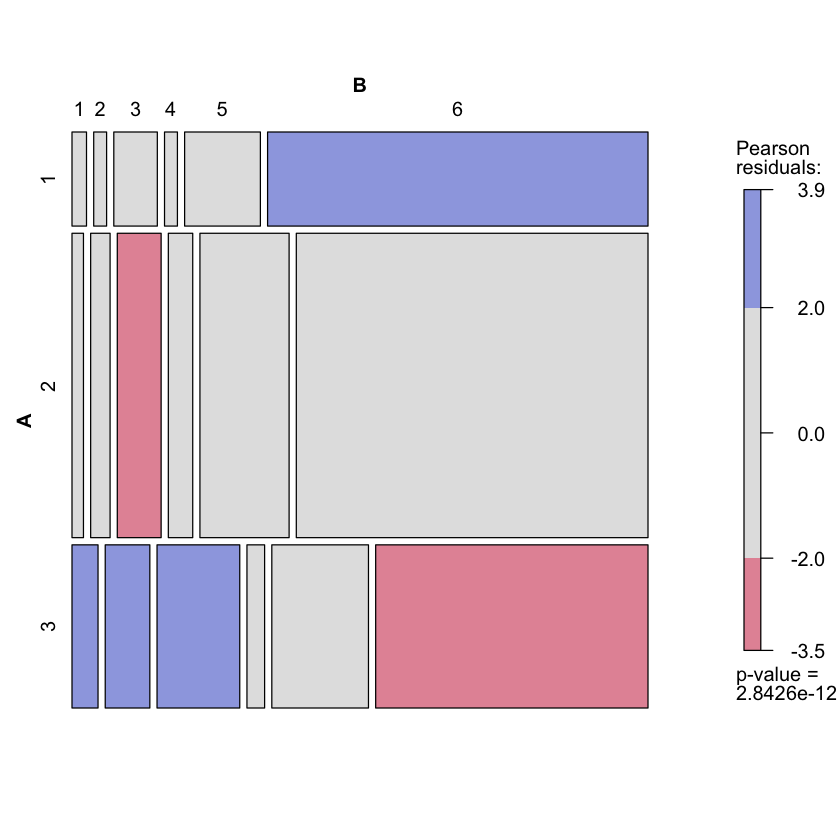
Visual representation of residuals
library(vcd)
mosaic(belief, shade=TRUE)
Loading required package: grid
Decomposition of LR stat
schizophrenia = matrix(c(90, 12, 78, 13, 1, 6, 19, 13, 50), 3, 3, byrow=TRUE) # Table 3.3
colnames(schizophrenia) = c('biogenic', 'environmental', 'combination')
rownames(schizophrenia) = c('eclectic', 'medical', 'psychoanalytic')
schizophrenia
lr_stat(schizophrenia)
| biogenic | environmental | combination | |
|---|---|---|---|
| eclectic | 90 | 12 | 78 |
| medical | 13 | 1 | 6 |
| psychoanalytic | 19 | 13 | 50 |
Warning message in chisq.test(data_table):
“Chi-squared approximation may be incorrect”
subtable = function(data_table, i, j) {
    new_table = matrix(0, 2, 2)
    for (k in 1:(i-1)) {
        for (l in 1:(j-1)) {
           new_table[1,1] = new_table[1, 1] + data_table[k, l]
        }
        new_table[1, 2] = new_table[1, 2] + data_table[k, j]
    }
    for (l in 1:(j-1)) {
        new_table[2, 1] = new_table[2, 1] + data_table[i, l]
    }
    new_table[2, 2] = data_table[i, j]
    return(new_table)
}
subtable(schizophrenia, 3, 3)
| 116 | 84 |
| 32 | 50 |
G_total = lr_stat(schizophrenia)
G_total
Warning message in chisq.test(data_table):
“Chi-squared approximation may be incorrect”
G_decomp = 0
for (i in 2:nrow(schizophrenia)) {
    for (j in 2:ncol(schizophrenia)) {
        increment = lr_stat(subtable(schizophrenia, i, j))
        print(increment)
        G_decomp = G_decomp + increment
    }
}
G_decomp
Warning message in chisq.test(data_table):
“Chi-squared approximation may be incorrect”
[1] 0.2941939
[1] 1.358793
[1] 12.95288
[1] 8.43033
What’s going on here?
Each
incrementis equal to LR test statistic comparing a simpler model to a richer one (this is not obvious at this point)Important: each of these models are nested: richer model at one stage becomes simpler model at next stage.
Each
incrementcan be written as $\( DEV(M_s) - DEV(M_r) \)\( where \)DEV\( is analogous to \)SSE$ inlm(we’ll see this more in next few weeks)Summing over the sequence yields telescoping sum which implies
G_decomp = G_total…For nested models \(M_0 \subset M_1 \subset \dots \subset M_k\) there is a decomposition of deviance analogous to a decomposition of SS (i.e. ANOVA)…
Fisher’s exact test for 2x2 tables
A test of \(H_0: \pi_{ij}=\pi_{i+} \pi_{+j}\) in one of the following models
\(N_{2 \times 2} \sim \text{Poisson}(\lambda_{2 \times 2})\) with \(\pi_{ij} = \lambda_{ij} / \sum_{k,l} \lambda_{k,l}\).
\(N_{2 \times 2} \sim \text{Multinomial}(N_{++}, \pi_{2 \times 2})\)
\(N_{i \cdot} \sim \text{Multinomial}(N_{1+}, \pi_{1, \cdot})\) independent across rows.
Conditional distribution
This is the distribution of the number of 1’s when drawing \(N_{1+}\) balls from a box with \(N_{+1}\) 1’s and \(N_{+2}\) 2’s.
tea_test = matrix(c(3, 1, 1, 3), 2, 2, byrow=TRUE) # Table 3.9
colnames(tea_test) = c('guess_milk', 'guess_tea')
rownames(tea_test) = c('truth_milk', 'truth_tea')
tea_test
fisher.test(tea_test, alternative='greater')
dhyper(3, 4, 4, 4) + dhyper(4, 4, 4, 4)
| guess_milk | guess_tea | |
|---|---|---|
| truth_milk | 3 | 1 |
| truth_tea | 1 | 3 |
	Fisher's Exact Test for Count Data

data:  tea_test
p-value = 0.2429
alternative hypothesis: true odds ratio is greater than 1
95 percent confidence interval:
 0.3135693       Inf
sample estimates:
odds ratio
  6.408309
Test can be generalized to \(I \times J\) tables but null distribution requires sampling (and naive MCMC does not work well c.f. Diaconis and Sturmfels)