LASSO
The LASSO adds a penalty to the objective
The indices for which \(\lambda_j=0\) are unpenalized.
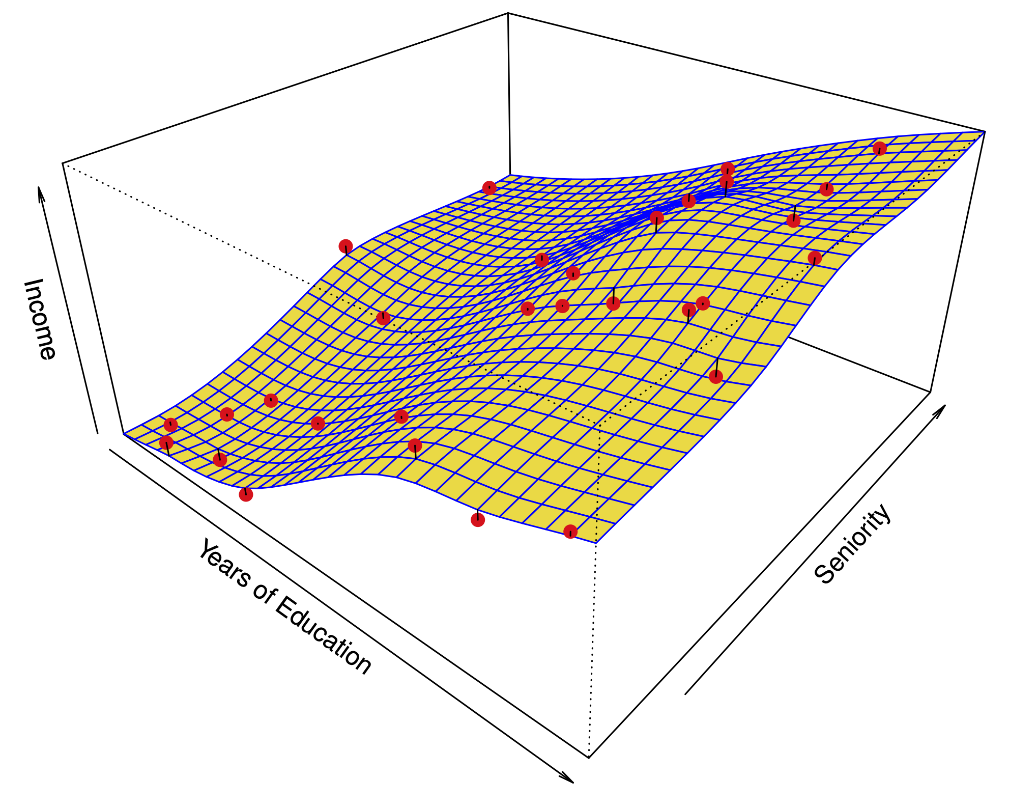
The LASSO picture

Why LASSO?
There are several sparsity inducing penalties out there: SCAD, MCP, etc.
But we know less about the “solutions” compared to LASSO because LASSO is a convex problem.
Solvable even in very high dimensions. (“same” for SCAD, MCP, etc.)
KKT conditions give an exact description of the solution however we decide to solve it (not same for SCAD, MCP, etc), at least under uniqueness.
Solving the LASSO
Many algorithms out there. Many of you will end up taking EE364 (Convex Optimization) where you’ll see things like this in more detail.
We’ll consider two simple algorithms: coordinate descent, proximal gradient descent.
Everyone has their own way of talking about LASSO. These notes are just my way.
Coordinate descent
If the penalty \({\cal P}\) were smooth, then we could use something like Newton-Raphson as we did for fitting the GLM.
The penalty is differentiable everywhere except points where one of the \(\beta_j\)’s is 0: \(\implies\) not smooth.
However, the penalty is separable meaning
Block separability allows for a partition of \(\{1,\dots,p\}= \cup_{g \in G} g\) – group LASSO an example of this.
When the penalty is separable, the problem can be solved by successively solving low-dimensional problems.
Basic iteration
Each iteration \(t\) chooses a coordinate \(j\) to update. Let the current position be \(\hat{\beta}^t\) define
Coordinate descent and Gibbs sampler
Suppose we have a prior with independent coordinates with negative log density \({\cal P}(\beta)\).
The Gibbs sampler considers same “objective” that a coordinate descent algorithm does.
Instead of minimizing this function, it draws from a density proportional to its negative exponential.
Each iteration \(t\) chooses a coordinate \(j\) to update. Let the current position be \(\hat{\beta}^t\) draw \(\hat{\beta}^{(t+1)}_j\) from a density proportional to:
Gibbs: sample
Coordinate Descent: optimize
Coordinate descent
coordinate_descent = function() {
    beta = rep(0, num_features)
    for (i in 1:enough_iterations) {
        for (j in 1:num_features) {
            cur_obj = objective(X, Y, penalty, "binomial", beta, j)
            beta[j] = argmax(cur_obj)
        }
    }
}
Gibbs sampler
gibbs_sampler = function() {
    beta = rep(0, num_features)
    for (i in 1:enough_iterations) {
        for (j in 1:num_features) {
            cur_post = objective(X, Y, prior, "binomial", beta, j)
            beta[j] = sample_univariate(exp(cur_post))
        }
    }
}
Logistic regression with offset
Each minimization is a logistic regression with a single feature \(X_j\) and offset \(X_{-j}\hat{\beta}^{(t)}_{-j}\).
Objective with offset vector \(Z\)
Stationarity conditions
Generally speaking offset \(Z\) shifts introduces affine predictor \(\beta \mapsto X\beta + Z\).
Example with offset
X_sim = matrix(rnorm(200), 100, 2)
Z_sim = rnorm(100)
Y_sim = rbinom(100, 1, 0.5)
M = glm(Y_sim ~ X_sim - 1, offset=Z_sim, family=binomial);
affine_pred = X_sim %*% coef(M) + Z_sim
pi_hat = exp(affine_pred) / (1 + exp(affine_pred))
t(X_sim) %*% (Y_sim - pi_hat)
| 3.587408e-15 |
| -7.105427e-15 |
At iteration \(t\), for each \(j\), if
then
Easy to check whether a coefficient should stay or be assigned to 0…
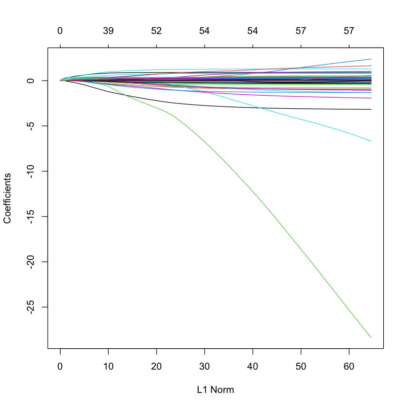
LASSO solution path for SPAM data
library(glmnet)
library(ElemStatLearn)
data(spam)
X_spam = scale(model.matrix(glm(spam ~ .,
                                family=binomial,
                                data=spam))[,-1]) # drop intercept
Y_spam = spam$spam == 'spam'
G_spam = glmnet(X_spam, Y_spam, family='binomial')
plot(G_spam)
Loading required package: Matrix
Loaded glmnet 4.0-2
Warning message:
“glm.fit: fitted probabilities numerically 0 or 1 occurred”
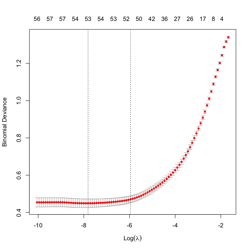
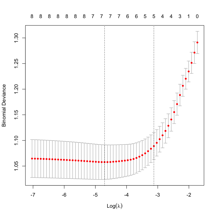
Cross-validation to choose \(\lambda\)
cvG_spam = cv.glmnet(X_spam, Y_spam, family='binomial')
plot(cvG_spam)
Re-solve at \(\lambda_{\min}\)
beta_CV_spam = coef(G_spam,
                    s=cvG_spam$lambda.min,
                    exact=TRUE,
                    x=X_spam,
                    y=Y_spam)
sum(beta_CV_spam[-1] != 0) # not very sparse in this case...
Predictions at new X
newX = X_spam[1:30,]
newY_hat = predict(G_spam,
	           newX,
                   s=cvG_spam$lambda.min,
                   type="response",
                   exact=TRUE,
                   x=X_spam,
                   y=Y_spam)
newY_hat[1:5]
- 0.573368457876324
- 0.979598740492402
- 0.999971117964625
- 0.747691413387677
- 0.747601439683215
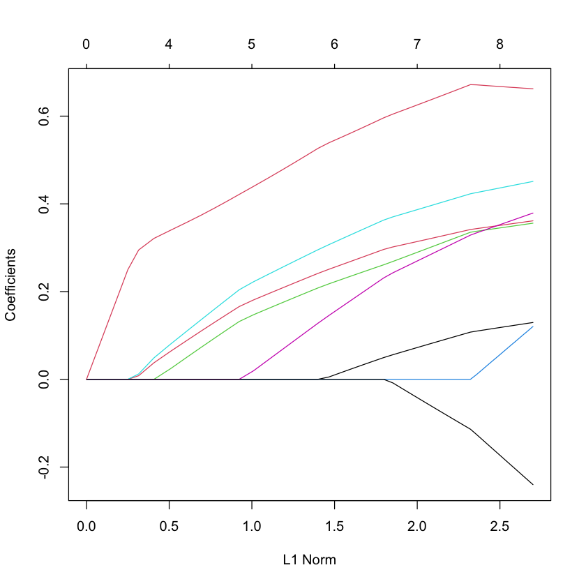
LASSO solution path for South African heart data
data(SAheart)
X_heart = scale(model.matrix(glm(chd ~ ., family=binomial, data=SAheart))[,-1]) # drop intercept
Y_heart = SAheart$chd
G_heart = glmnet(X_heart, Y_heart, family='binomial')
plot(G_heart)
Cross-validation to choose \(\lambda\)
cvG_heart = cv.glmnet(X_heart, Y_heart, family='binomial')
plot(cvG_heart)
Re-solve at \(\lambda_{1SE}\)
beta_1se_heart = coef(G_heart,
                      s=cvG_heart$lambda.1se,
                      exact=TRUE,
                      x=X_heart,
                      y=Y_heart)
sum(beta_1se_heart[-1] != 0) # eliminates a few
Proximal gradient descent
Updates all coordinates each step.
This method takes advantage of the fact that
is soft-thresholding, most importantly it is fast
Solution is
Basic update
Given current state \(\hat{\beta}^{(t)}\) define
The next iterate is defined as
Comments
Quadratic approximation similar to Newton-Raphson.
If \(L\) is chosen so that \(L \cdot I \geq \nabla^2 \ell(\beta)\) for all \(\beta\) then this is an example of Majorization-Minimization (MM) method.
Stepsize \(L\) only needs to be chosen to be a descent – backtracking typically used.
There are several accelerated proximal gradient descent algorithms out there, some local to us: NESTA, TFOCS.
Proximal algorithm is key ingredient to all of these methods.
Majorization-Minimization
Suppose we want to solve
We assume we have a function \(M(\beta;\beta')\) such that
Set
Then, \(f(\hat{\beta}^{(t+1)}) \leq f(\hat{\beta}^{(t)})\). Yields a descent method!
Gradient descent and Langevin sampler
Just as coordinate descent “looks” like Gibbs sampling. There is an analogous MCMC sampler (at least for smooth penalties…)
Langevin sampling
with \(\xi^{(t)} \sim N(0,I)\).
Reference: e.g. Dalalyan
Proximal map
The map
is called the proximal operator of \({\cal P}\).
Proximal gradient descent methods rely on \({\cal P}\) being fast.
Each step above evaluates the proximal map of \(L^{-1} \cdot {\cal P}\).
Reference: Parikh and Boyd
Solving the LASSO
LASSO in bound form
Original LASSO:
subject to \({\cal P}(\beta) \leq C\).
Proximal gradient descent replaces soft-thresholding with map
Solving LASSO in this form will repeatedly project
onto the convex set \(\left\{\beta: \|\beta\|_1 \leq C \right\}.\)
KKT conditions
How will we know we have solved
KKT conditions read
where
The set \(\partial {\cal P}(\beta)\) is called the subdifferential of \({\cal P}\) at \(\beta\).
If \({\cal P}\) is differentiable at \(\beta\), then the subdifferential is the derivative.
Can also deduce stationarity conditions from proximal gradient algorithm.
Stationarity from proximal gradient
If \(\hat{\beta}\) is a statitionary point of proximal gradient with step size \(L^{-1}\), then
If \(\hat{\beta}_i=0\) then
If \(\hat{\beta}_i \neq 0\) then
Very briefly, what is the subdifferential for our \({\cal P}\)?
Note that
For penalties of the form
the subdifferential is
with \(N_u(K)\) the set of normal directions at \(u \in K\).
Also characterized as
Normal cones of a cube

Suppose \(\hat{\beta}_{-E}=0, \min_{j \in E}|\hat{\beta}_j|>0\) and \(\text{sign}(\hat{\beta}_E)=s_E\).
Then,
In other words: active signs are fixed, inactive score is not too big.
X = matrix(rnorm(300), 100, 3)
beta = rep(0, 3)
beta[1:2] = 3
Y = X %*% beta + rnorm(100)
G = glmnet(X, Y, standardize=FALSE, intercept=FALSE)
lam = G$lam[10]
lam
beta_hat = coef(G, s=lam, exact=TRUE, x=X, y=Y)[2:4]
beta_hat
- 1.75879739460179
- 1.60004492874385
- 0
score = (t(X) %*% (X %*% beta_hat - Y) / 100)
score
lam
| -1.44969577 |
| -1.44969589 |
| 0.01360631 |
c(beta_hat[1:2], score[3])
- 1.75879739460179
- 1.60004492874385
- 0.0136063095635466
Let’s perturb \(Y\) a little and see what happens.
Y_star = Y + 0.1 * rnorm(100)
G_star = glmnet(X, Y_star, intercept=FALSE, standardize=FALSE)
beta_star = coef(G_star, s=lam, exact=TRUE, x=X, y=Y_star)[2:4]
beta_star
- 1.75907492754101
- 1.60473445347705
- 0
score_star = t(X) %*% (X %*% beta_star - Y_star) / 100
score_star
| -1.44969498 |
| -1.44969589 |
| 0.01240643 |
c(beta_star[1:2], score_star[3])
c(beta_hat[1:2], score[3])
- 1.75907492754101
- 1.60473445347705
- 0.0124064281382372
- 1.75879739460179
- 1.60004492874385
- 0.0136063095635466
KKT conditions: deeper dive
Restricted problem
Suppose variables \(E\) are selected with signs \(s_E\).
KKT equations yield
Having fixed \(E\) we can define restricted objective
First equation reads
with constraint \(\text{sign}(\hat{\beta}_E) = s_E\).
Gaussian case
Let’s take one Newton-Raphson step from \(\hat{\beta}_E\):
or
In the Gaussian case this reads $\( \text{sign}((X_E'X_E)^{-1}(X_E'Y - \lambda_E s_E)) = s_E. \)$
Allowing some \(\lambda_i\)’s to be zero changes things a little – only have conditions for \(\lambda_i > 0\).
Inactive block
Let’s look at our other set of KKT equations.
We know that
For any fixed \(E\), \(\nabla \ell(\bar{\beta}_E, 0)_{-E}\) will by asymptotically Gaussian under standard conditions. It will have mean 0 if the model \(E\) is correctly specified.
The vector
will behave as a fixed vector (with signs fixed).
Gaussian case
Model selection consistency
Now suppose that model is correct with parameter \(\beta^*\) such that \(\beta^*_{-A}=0\).
When will the LASSO recover \(A\) with correct signs \(\text{sign}(\beta^*_A)\)? (For simplicity let’s now set all \(\lambda_i\)’s equal).
References (among others): Zhao and Yu, Candes and Plan
Our look at the active block of the KKT conditions says that if we solve the restricted MLE on \(A\) and we shrink we must still have the same signs.
Up to small remainder this event is
with \(s^*_A=\text{sign}(\beta^*_A)\).
If \(\beta_A^*\) are far away enough from 0 (beta-min condition) then subtracting the second term will not change signs of \(\bar{\beta}_A\).
Let’s look at the inactive block. We saw that if the active set is going to be \(A\) and signs \(s_A^*\) then
For this to happen, essentially we need the irrepresentable condition (Zhao and Yu)
How large should \(\lambda\) be?
The irrepresentable condition suggests \(\lambda\) should be such that $\( \|\nabla \ell(\bar{\beta}_A, 0)_{-A}/\lambda\|_{\infty} < 1. \)$
A typical choice
Such choice often guarantees LASSO is consistent. (Large literature on this, c.f. Negabhan et al.)