Linear models
We’ve seen several linear models in the course, most likelihood based…
Generic setup: independent \(Y_i\)’s parameterized by \(\eta_i\).
Linear model imposes \(\eta_i=X_i^T\beta\).
Deviance (-2 log likelihood) provides objective function to estimate \(\beta\).
These models have nice structure when \(Y_i\)’s are from some exponential family: often convex (negative log-likelihoods) which make it easy to regularize, go to high dimensions, etc.
Likelihoods we’ve looked at
Binomial
Poisson
Multinomial
Cox partial likelihood
Other models: multivariate Gaussian
Setup: \(Y_{n \times q}\), \(X_{n \times p}\)
Model: \(Y|X \sim N(XB, I_{n \times n} \otimes \Sigma_{q \times q})\) for \(B_{p \times q}\) (covariance is multivariate Kronecker notation for IID draws from \(N(0,\Sigma)\).
A likelihood based model: MLE (exactly analogous to univariate reponse):
Can regularize in groups for group sparsity
Other models: robust regression rlm
Setup: \(Y_{n \times 1}\), \(X_{n \times p}\)
Model: typically not thought of as a likelihood…
Estimator:
Other models: robust regression rlm

Examples of \(\rho\): \(\ell_1\), Huber, Tukey biweight or other redescending estimator.
Regularization? Sure… (Huber and \(\ell_1\) are at least convex…)
Other models: quantile regression
Consider \(\ell_1\):
Instead of modeling \(E[Y|X]\) this models \(\text{median}(Y|X)\).
Pinball loss: \(\tau \in (0,1)\)
Models the \(\tau\)-quantile of \(Y|X\).
Other models: robust regression rlm

Score equations
Inference? Sandwich or bootstrap.
Other models: support vector machine (SVM)

Not always phrased this way, but equivalent to using hinge loss
For binary outcome \(Y\) coded as \(\pm 1\) and linear predictor \(\eta\)
Huberized SVM smooths out this loss as Huber does the \(\ell_1\) (Moreau smoothing)
Other models: support vector machine (SVM)
Regularization: convex in \(\eta\) so, sure…
Inference? Bootstrap?
Mixed effects models
Setup: \(Y_{n \times 1}\), \(X_{n \times p}\)
Model: \(Y|X \overset{D}{=} X\beta + Z\gamma + \epsilon\)
Measurement error \(\epsilon \sim N(0, \sigma^2 I)\)
Random effect (usually independent of \(\epsilon\)) \(\gamma \sim N(0, \Sigma(\theta))\).
Mixed effects models
Log-likelihood
Estimation: not convex but smooth…
Inference: likelihood based (if you believe the model)
Mixed effects models: estimation
EM algorithm (if we observed \(\gamma\)) likelihood would be nice and simple.
Gradient descent…
Messy, but feasible to run Newton-Raphson…
Since we have a likelihood, Bayesian methods are applicable here.
Mixed effects models: REML
REML: notes that law of residuals does not depend on \(\beta\)
Decomposes problem into noise parameter estimation and fixed effects estimation.
This likelihood can be used to estimate \((\theta,\sigma^2)\).
Given this estimate \((\widehat{\sigma}^2, \widehat{\theta})\) the optimal \(\beta\) is
REML is often a better estimate than MLE for noise: in usual Gaussian model \(\widehat{\sigma}^2_{REML} = \|Y-X\widehat{\beta}\|^2_2/(n-p)\)…
Generalized linear mixed models
Gaussian mixed effects model essentially models linear predictor
Lends itself naturally to
glmlikelihoods as well.E.g. for Binomial data with logistic link
Generalized linear mixed models
Likelihood marginalizes over \(\gamma\) – no closed form (unlike Gaussian model).
Many computational issues to deal with here.
Well suited to Bayesian modeling here (though if optimization is difficult, likely that posteriors are quite multi-modal for non-informative priors…)
Beyond linear models: basis expansions
We’ve always used linear predictor
Could use a basis expansion with \(N_j\) functions for feature \(j\)
Any linear method that takes linear predictor can profit from basis expansion.
Generally, these form additive models
Implicit basis expansions
As basis expansion grows in complexity we should regularize in some fashion…
For explicit basis, we could choose sparsity or some ridge
Kernel trick
A natural class of penalties
A covariance function \(K:\mathbb{R} \times \mathbb{R} \rightarrow \mathbb{R}\) is a function that satisfies:
\(K(s,t)=K(t,s)\) (symmetry)
For any \(\{t_1, \dots, t_k\} \subset\mathbb{R}\) and coefficients \(\{a_1, \dots, a_k\}\) we have \(\sum_{i,j=1}^k a_i a_j K(t_i, t_j)>0\). (non-negative definite)
Example: radial basis function \(K(t,s) = e^{-(t-s)^2/(2\gamma)}\).
Example: Brownian motion \(K(t,s) = \min(t,s)\).
Reproducing kernel penalty
Consider functions of the form:
The penalty is
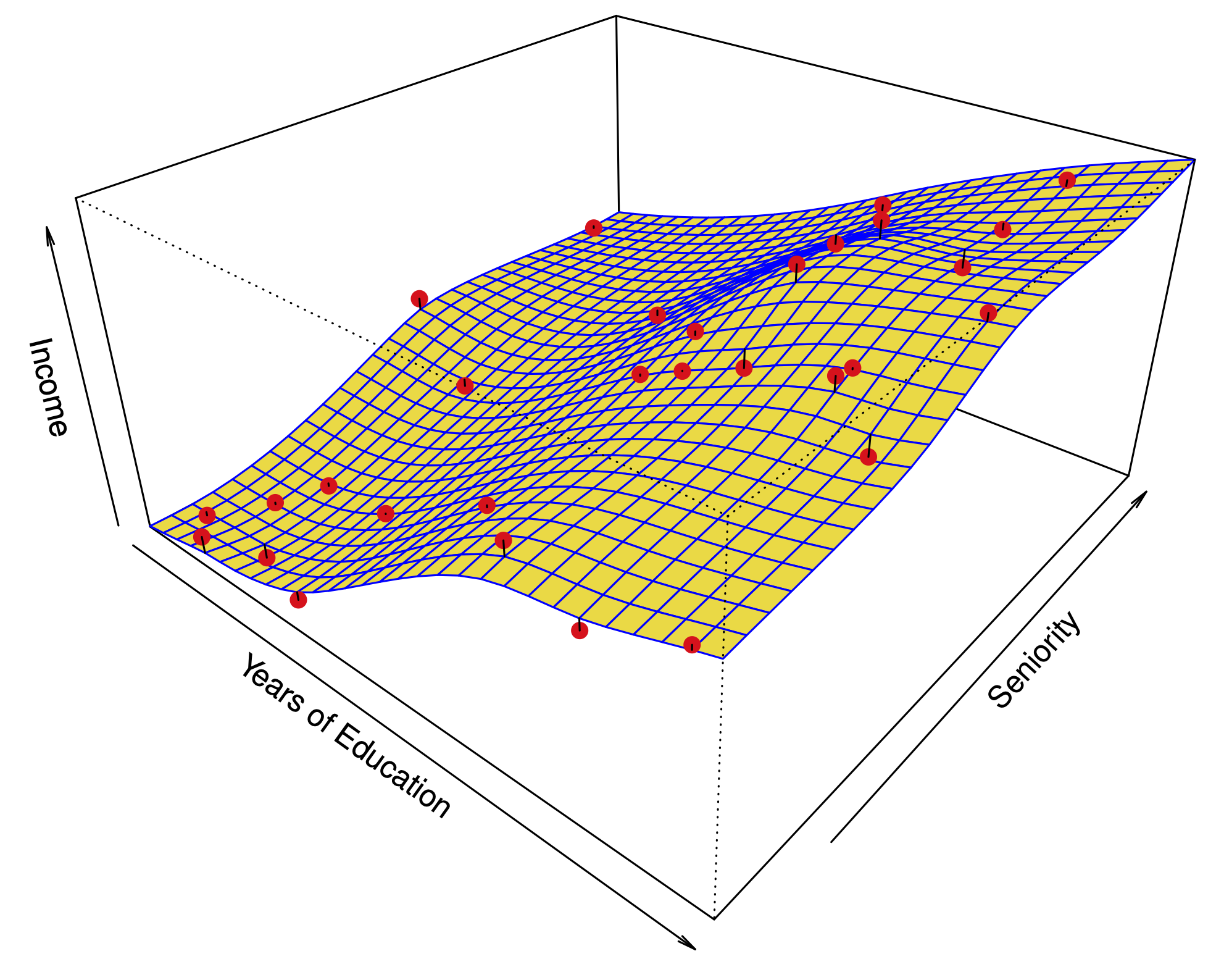
Penalized regression
Kernels can take multivariate arguments \(K:\mathbb{R}^k \times \mathbb{R}^k \rightarrow \mathbb{R}\).
Greatly expands flexibility of regression modelling…. (at cost of having more choices to make!)
Combining ideas
Kernel trick tells us how to make lots of cool feature mappings…
Can be plugged into other regression problems, e.g. “non-parametric” quantile regression
“Non-parametric” survival analysis