Penalized regression
The objective function for a GLM (as a minimization) can be written as
With some abuse of notation
and \(\Lambda\) is the log MGF of \(Y\)’s as a function of the natural parameter.
Penalized regression
Objective:
Three examples we’ve seen:
Gaussian \(\Lambda(\alpha) = \alpha^2/2\) (or scale objective \(\sigma^2\));
Logistic \(\Lambda(\alpha) = \log(1 + e^{\alpha})\).
Poisson log-linear \(\Lambda(\alpha) = e^{\alpha}\).
Ridge regression
Ridge regression adds a quadratic pnalty
Estimator
Features are usually centered and scaled so coefficients are unitless.
“Bayesian” interpretation
If we were to put a \(N(0, \lambda^{-1} I)\) prior on \(\beta\) its log posterior would be (up to normalizing constant depending only on \((X,Y)\))
Ridge estimator yields MAP (Maximum A Posteriori) estimator (i.e. the posterior mode).
Easy to add weights
unpenalized variables have \(\lambda_j=0\).
General quadratics also fine
Corresponds to \(N(0,Q^{-1})\) prior.
Overall objective
Solving for the ridge estimator
From unpenalized case we know 2nd Taylor approximation of likelihood.
Differentiating the penalty:
Newton-Raphson / Fisher scoring
For canonical models
General form
Not the only way to solve this problem…
Why do we regularize?
Consider Gaussian case with \(Q=\lambda I\)
Writing \(X=UDV'\) we see
Bias
Writing \(\beta=\sum_j \alpha_j V_j\):
Variance
RHS is trace of \(\text{Var}((X'X)^{-1}(X'Y))\).
Ridge always has smaller variance.
MSE
Assuming \(\beta \neq 0\)
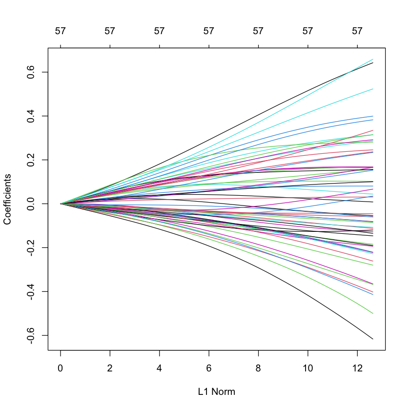
Ridge solution path for SPAM data
library(glmnet)
library(ElemStatLearn)
data(spam)
X_spam = scale(model.matrix(glm(spam ~ .,
                                family=binomial,
                                data=spam))[,-1]) # drop intercept
Y_spam = spam$spam == 'spam'
G_spam = glmnet(X_spam,
                Y_spam,
                alpha=0, # this makes it ridge
                family='binomial')
plot(G_spam)
Loading required package: Matrix
Loaded glmnet 4.0-2
Warning message:
“glm.fit: fitted probabilities numerically 0 or 1 occurred”
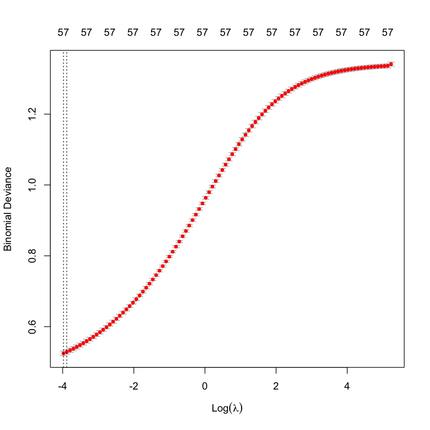
Cross-validation to choose \(\lambda\)
cvG_spam = cv.glmnet(X_spam,
                     Y_spam,
                     alpha=0,
                     family='binomial')
plot(cvG_spam)
Re-solve at \(\lambda_{\min}\)
beta_CV_spam = coef(G_spam,
                    s=cvG_spam$lambda.min,
                    exact=TRUE,
                    x=X_spam,
                    y=Y_spam,
                    alpha=0)
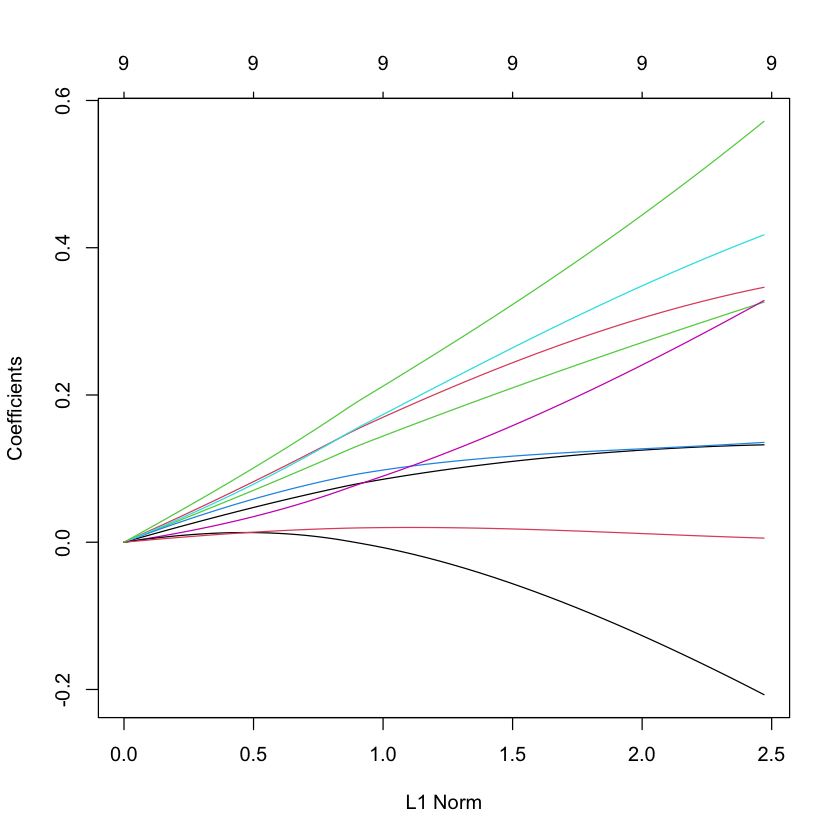
Ridge solution path for South African heart data
data(SAheart)
X_heart = scale(model.matrix(glm(chd ~ ., family=binomial, data=SAheart))[,-1]) # drop intercept
Y_heart = SAheart$chd
G_heart = glmnet(X_heart,
                 Y_heart,
                 alpha=0,
                 family='binomial')
plot(G_heart)
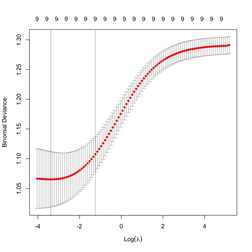
Cross-validation to choose \(\lambda\)
cvG_heart = cv.glmnet(X_heart,
                      Y_heart,
                      alpha=0,
                      family='binomial')
plot(cvG_heart)
Re-solve at \(\lambda_{1SE}\)
beta_1se_heart = coef(G_heart,
                      s=cvG_heart$lambda.1se,
                      exact=TRUE,
                      alpha=0,
                      x=X_heart,
                      y=Y_heart)