From discrete to continuous: Lindsey’s method
For ordinal discrete \(X^D\) we considered at least two models:
Saturated: \(\lambda_i\) unconstrained
Ordinal with scores: \(\lambda_i = \beta_0 + \beta_1 \cdot i\)
Continuous
Suppose \(X\) is a continuous random variable supported on \([0,1]\) and we discretize
Our ordinal model for such \(X^{\Delta}\) looks like
Corresponds to a density of the form
When fitting a loglinear GLM to \(X^{\Delta}\) with \(\Delta\) small we should have (assuming the density is well-specified)
Basis expansion
No reason to restrict scores to just be \(i\)…
Can extend from \([0,1]\) to all of \(\mathbb{R}\) by adding “bins” of the form \([C,\infty)\) and \((-\infty,C]\) (with unrestricted parameters)
Thinking of index as \(i \cdot \Delta\) consider a model
This is a discretization of a density
Taking \(h_1(x)=x, h_2(x)=x^2\) we arrive at (discretization) of a Gaussian.
Custom families: Lindsey’s method
Bins need not be of same size – correspond to an offset in a GLM.
“Representative point” of a bin need not be the right hand endpoint, could be midpoint, left end point….
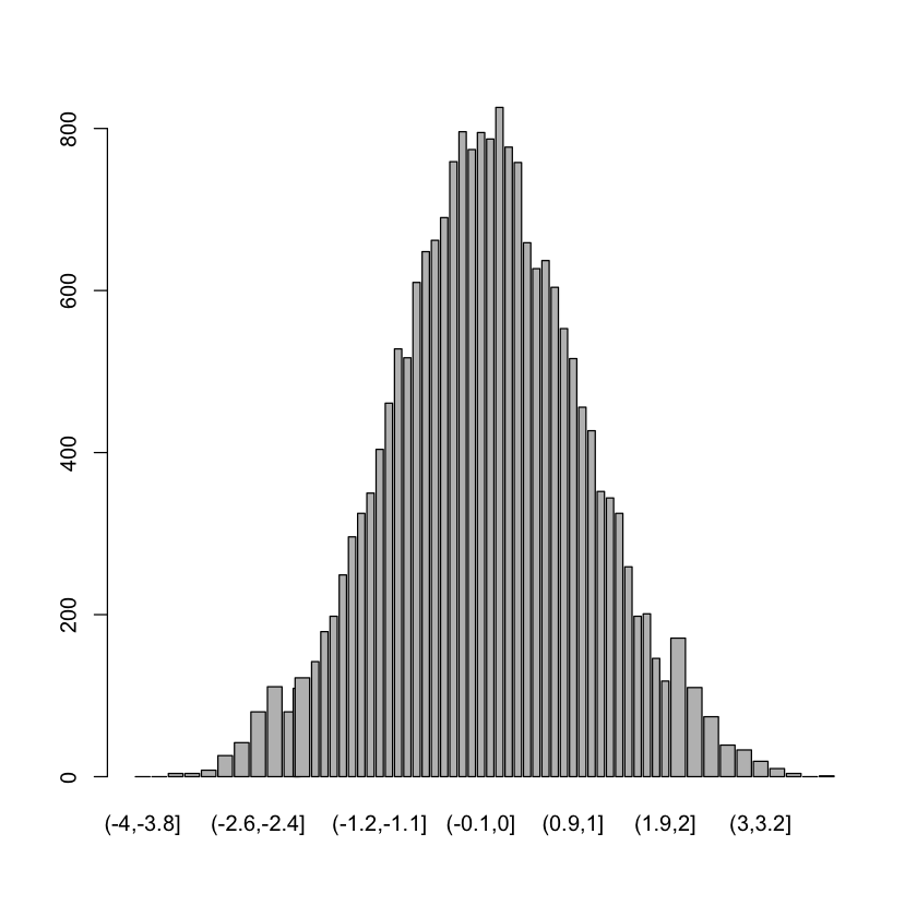
X = rnorm(20000)
bins = unique(c(seq(-4,-2,by=0.2),
                seq(-2.1,2,by=0.1),
                seq(2.2, 4, by=0.2)))
Y = table(cut(X, breaks=bins))
midpts = (bins[1:(length(bins)-1)] + bins[2:length(bins)])/2
widths = bins[2:length(bins)] - bins[1:(length(bins)-1)]
barplot(Y, widths)
df = cbind(Y, midpts, midpts^2)
colnames(df) = c('N', 'linear', 'quadratic')
df = data.frame(df)
M = glm(N ~ linear + quadratic,
        family=poisson,
        offset=log(widths),
        data=df)
Warning message in log(widths):
“NaNs produced”
summary(M)
Call:
glm(formula = N ~ linear + quadratic, family = poisson, data = df,
    offset = log(widths))

Deviance Residuals:
    Min       1Q   Median       3Q      Max
-7.0377  -0.5934   0.1681   0.9296   2.3041

Coefficients:
             Estimate Std. Error  z value Pr(>|z|)
(Intercept)  8.981528   0.008706 1031.682  < 2e-16 ***
linear       0.027773   0.007092    3.916 8.99e-05 ***
quadratic   -0.507006   0.005051 -100.382  < 2e-16 ***
---
Signif. codes:  0 ‘***’ 0.001 ‘**’ 0.01 ‘*’ 0.05 ‘.’ 0.1 ‘ ’ 1

(Dispersion parameter for poisson family taken to be 1)

    Null deviance: 26759.61  on 59  degrees of freedom
Residual deviance:   154.95  on 57  degrees of freedom
  (1 observation deleted due to missingness)
AIC: 560.24

Number of Fisher Scoring iterations: 4
M_no_offset = glm(N ~ linear + quadratic,
        family=poisson,
        data=df)
summary(M_no_offset)
Call:
glm(formula = N ~ linear + quadratic, family = poisson, data = df)

Deviance Residuals:
    Min       1Q   Median       3Q      Max
-2.9386  -1.2079  -0.1816   0.9336   4.5798

Coefficients:
             Estimate Std. Error z value Pr(>|z|)
(Intercept)  6.635284   0.008815 752.716  < 2e-16 ***
linear       0.018348   0.007010   2.618  0.00886 **
quadratic   -0.431763   0.005172 -83.482  < 2e-16 ***
---
Signif. codes:  0 ‘***’ 0.001 ‘**’ 0.01 ‘*’ 0.05 ‘.’ 0.1 ‘ ’ 1

(Dispersion parameter for poisson family taken to be 1)

    Null deviance: 16321.28  on 60  degrees of freedom
Residual deviance:   184.92  on 58  degrees of freedom
AIC: 596.75

Number of Fisher Scoring iterations: 4
Joint distributions
Suppose \((X,Y)\) are two discrete ordinal variables and \(N_{ij} \sim \text{Poisson}(\lambda_{ij})\) is an \(I\times J\) contingency table representing a sample from \((X,Y)\).
Ordinal (independence): \(\lambda_{ij} = \beta_0 + \beta_X i + \beta_Y j\).
Ordinal with dependence?: \(\lambda_{ij} = \beta_0 + \beta_X i + \beta_Y j + \beta^{XY}_{ij}\).
Back to discretization
Suppose \((X^{\Delta}, Y^{\Delta})\) are such discretizations
Basis expansion (independence): \(\lambda_{ij} = \gamma_0 + \sum_j \gamma^X_j h^X_j(i\Delta) + \sum_l \gamma^Y_l h_l^Y(j\Delta)\)
What about dependence?
Add a term of the form
Dependence modeled by matrix \(\gamma^{XY}\).
What kind of \(h^{XY}\)?
Convenient to consider tensor products \(h^{XY}_{j'l'} = g^X_{j'l'}(x) g^Y_{j'l'}(y)\).
Example: if we set \(h^X_1(s)=h^Y_1(s)=s, h^X_2(s)=h^Y_2(s)=s^2\) and \(h^{XY}_{11}(x,y)=xy\) \(\implies\) Gaussian!
Use of tensor products can make conditionals nice (i.e. “simpler” pseudo-likelihood).
Mix of discrete and Gaussian
Suppose \(X\) is continuous and \(Y\) is discrete with \(K\) levels
For “main effects” of \(X\) we take \(h^X_1(x)=x, h^X_2(x)=x^2\).
For “main effects” of \(Y\) we take one-hot encoding \(h^Y_k(y) = \delta_j(y), 1 \leq k \leq K\).
For “interactions” we take \(h^{XY}_{1k}(x,y) = x \cdot \delta_k(y)\) – tensor product of (some) terms in the “main effect”. (Could also have the variance change as well.)
\(\implies\) conditionals \(X|Y\) and \(Y|X\) will be in the same family as implied by “main effect”.
\(X|Y\) is Gaussian (equivalent to
lm(X ~ factor(Y)))\(Y|X\) is multinomial (equivalent to a baseline multinomial logit
nnet::multinom(Y ~ X)).
Parameters
The “interactions” are encoded by \(\gamma_{1,k} \in \mathbb{R}^{1 \times K}\).
Two discrete variables
Suppose \(Z\) is discrete with \(L\) levels and \(Y\) is discrete with \(K\) levels
For “main effects” of \(Z\) we take one-hot encoding \(h^Z_l(l)=\delta_l(z) , 1 \leq l \leq L\).
For “main effects” of \(Y\) we take one-hot encoding \(h^Y_k(y) = \delta_j(y), 1 \leq k \leq K\).
For “interactions” we take \(h^{ZY}_{lk}(z,y) = \delta_l(z) \delta_k(y)\) – tensor product of terms in the “main effect”.
Parameters
The “interactions” are encoded by \(\gamma_{l,k} \in \mathbb{R}^{L \times K}\).
Several continuous and discrete variables
For all continuous variables use the Gaussian encoding with \(x \mapsto x, x \mapsto x^2\) as main effects.
For all discrete variables use the one-hot encoding \(x \mapsto \delta_l(x)\)
Interactions
Use the tensor product formulation, but for any continuous interactions use only the \(x \mapsto x\) main effect.
Continuous / continuous: a single parameter \(\mathbb{R}\)
Continuous / discrete with \(L\) levels: a vector \(\mathbb{R}^L\)
Discrete with \(L\) levels / discrete with \(K\) levels: a matrix in \(\mathbb{R}^{L \times K}\).
Pseudo-likelihoods
For every continuous variable: Gaussian linear model
For every discrete variable: baseline multinomial logit
Conditional independence
Absence of any interaction \(\implies\) conditional independence.
Selecting edges: group LASSO
Want a penalty that can zero-out an entire vector (continuous / discrete) or matrix (discrete / discrete).
Consider
For matrices use Frobenius (Euclidean norm of matrix entries)
Combine with pseudo-likelihood and proximal gradient and away we go…