Poisson data (4.3)
Suppose \(Y \sim \text{Poisson}(\lambda)\).
Then, for \(y=0,1,2, \dots\)
This is one-parameter exponential family with sufficient statistic \(y\), natural parameter \(\log \lambda\), \(b(y)=1/y!\) and \(m\) counting measure on \(\{0,1,2,\dots\}\).
Generalized linear models for counts
Poisson is a natural model for counts (arguably, we might say this is because it appears in many limiting arguments involving counts).
Given \((Y_i,X_i)\) with \(Y_i \sim Poisson(\lambda_i)\), the log-linear model is
with
Just as there is a canonical link for Binomial data, there is one for Poisson as well. (What is canonical link for Gaussian?)
The log link here is related to conditional independencies among features \(X\) and response \(Y\).
Note that for Poisson data $\( \text{Var}[Y_i|X_i] = \lambda_i. \)$
Interpretation of coefficients
Likelihood for log-linear models
The Poisson deviance for the log-linear model is $\( DEV(\beta|Y) = 2 \sum_{i=1}^n \left[\exp(X_i^T\beta) - Y_i(X_i^T\beta) - Y_i + Y_i \log(Y_i) \right] \)$
Derivatives
Similar form to logistic regression.
library(glmbb) # for `crabs` data
data(crabs)
satell_log = glm(satell ~ width + color, family=poisson(), data=crabs)
summary(satell_log)
Call:
glm(formula = satell ~ width + color, family = poisson(), data = crabs)

Deviance Residuals:
    Min       1Q   Median       3Q      Max
-3.0415  -1.9581  -0.5575   0.9830   4.7523

Coefficients:
            Estimate Std. Error z value Pr(>|z|)
(Intercept) -3.08640    0.55750  -5.536 3.09e-08 ***
width        0.14934    0.02084   7.166 7.73e-13 ***
colordarker -0.01100    0.18041  -0.061   0.9514
colorlight   0.43636    0.17636   2.474   0.0133 *
colormedium  0.23668    0.11815   2.003   0.0452 *
---
Signif. codes:  0 ‘***’ 0.001 ‘**’ 0.01 ‘*’ 0.05 ‘.’ 0.1 ‘ ’ 1

(Dispersion parameter for poisson family taken to be 1)

    Null deviance: 632.79  on 172  degrees of freedom
Residual deviance: 559.34  on 168  degrees of freedom
AIC: 924.64

Number of Fisher Scoring iterations: 6
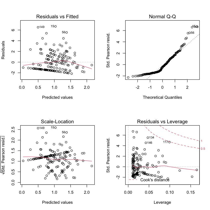
par(mfrow=c(2,2))
plot(satell_log)
Newton-Raphson for log-linear models
After initialization $\( \hat{\beta}^{(k+1)} = \hat{\beta}^{(k)} + (X^T\exp(X\hat\beta^{(k)})X)^{-1} X^T(Y - \exp(X\hat\beta^{(k)})) \)$
Can be written as IRLS with weights and response
“Unnatural models”
We could use a different link function
or,
Deviance is now
Usual choices in software for Poisson is
log(canonical: default). Others:identity: \(g(x)=x\)inverse: \(g(x)=1/x\).
satell_inverse = glm(satell ~ width + color,
                     family=poisson(link='inverse'),
                     data=crabs)
summary(satell_inverse)
Call:
glm(formula = satell ~ width + color, family = poisson(link = "inverse"),
    data = crabs)

Deviance Residuals:
    Min       1Q   Median       3Q      Max
-2.8701  -2.0606  -0.4481   1.0042   4.6942

Coefficients:
             Estimate Std. Error z value Pr(>|z|)
(Intercept)  1.259804   0.136929   9.200  < 2e-16 ***
width       -0.031806   0.004905  -6.484 8.92e-11 ***
colordarker  0.011778   0.077006   0.153   0.8784
colorlight  -0.126441   0.055752  -2.268   0.0233 *
colormedium -0.085615   0.045740  -1.872   0.0612 .
---
Signif. codes:  0 ‘***’ 0.001 ‘**’ 0.01 ‘*’ 0.05 ‘.’ 0.1 ‘ ’ 1

(Dispersion parameter for poisson family taken to be 1)

    Null deviance: 632.79  on 172  degrees of freedom
Residual deviance: 574.53  on 168  degrees of freedom
AIC: 939.82

Number of Fisher Scoring iterations: 8
“Unnatural models”
Derivatives
with
“Unnatural models”
Fisher scoring $\( \hat{\beta}^{(k+1)} = \hat{\beta}^{(k)} + (X^TW_{\hat{\beta}^{(k)}}X)^{-1}X^T\left(\frac{1 - \frac{Y}{E_{\beta}(Y)}}{g'(E_{\beta}(Y))}\right) \)$
Equivalent to IRLS with
with
Form of weights comes from “\(\text{Var}(Z)\)”.
Recall that \(E_{\beta}(Y)=\text{Var}_{\beta}(Y)\) for Poisson data.
Distribution of \(\hat{\beta}\)
Using our usual Taylor series $\( \hat{\beta} - \beta^* \approx N\left(0, (X^TW^{(\infty)}X)^{-1} \text{Var}(X^TW^{(\infty)}Z^{(\infty)})(X^TW^{(\infty)}X)^{-1} \right) \)$
When model is correct, $\( \text{Var}(X^TW^{(\infty)}Z^{(\infty)}) \approx X^TW^{(\infty)}X \)\( so asymptotic distribution is \)\( \hat{\beta} - \beta^* \approx N\left(0, (X^TW^{(\infty)}X)^{-1} \right). \)$
This is covariance that
Rreports to us withvcov.
X = model.matrix(satell_log)
W = fitted(satell_log)
solve(t(X) %*% (W * X))
| (Intercept) | width | colordarker | colorlight | colormedium | |
|---|---|---|---|---|---|
| (Intercept) | 0.310805970 | -0.0114263483 | -0.0162473663 | 0.0019301044 | 0.0027713727 |
| width | -0.011426348 | 0.0004343334 | 0.0002297147 | -0.0004612394 | -0.0004932173 |
| colordarker | -0.016247366 | 0.0002297147 | 0.0325477977 | 0.0099601366 | 0.0099432238 |
| colorlight | 0.001930104 | -0.0004612394 | 0.0099601366 | 0.0311020571 | 0.0107278527 |
| colormedium | 0.002771373 | -0.0004932173 | 0.0099432238 | 0.0107278527 | 0.0139590542 |
vcov(satell_log)
| (Intercept) | width | colordarker | colorlight | colormedium | |
|---|---|---|---|---|---|
| (Intercept) | 0.310805898 | -0.0114263456 | -0.0162473648 | 0.0019301016 | 0.0027713695 |
| width | -0.011426346 | 0.0004343333 | 0.0002297147 | -0.0004612393 | -0.0004932172 |
| colordarker | -0.016247365 | 0.0002297147 | 0.0325477151 | 0.0099601366 | 0.0099432238 |
| colorlight | 0.001930102 | -0.0004612393 | 0.0099601366 | 0.0311020569 | 0.0107278525 |
| colormedium | 0.002771369 | -0.0004932172 | 0.0099432238 | 0.0107278525 | 0.0139590539 |
X = model.matrix(satell_inverse)
W = fitted(satell_inverse)^3
solve(t(X) %*% (W * X))
| (Intercept) | width | colordarker | colorlight | colormedium | |
|---|---|---|---|---|---|
| (Intercept) | 0.0187471088 | -6.400857e-04 | -2.108431e-03 | -7.723414e-04 | -1.139935e-04 |
| width | -0.0006400857 | 2.405665e-05 | 1.474627e-05 | -3.546863e-05 | -6.021163e-05 |
| colordarker | -0.0021084309 | 1.474627e-05 | 5.933203e-03 | 1.694329e-03 | 1.679162e-03 |
| colorlight | -0.0007723414 | -3.546863e-05 | 1.694329e-03 | 3.108126e-03 | 1.804845e-03 |
| colormedium | -0.0001139935 | -6.021163e-05 | 1.679162e-03 | 1.804845e-03 | 2.092418e-03 |
vcov(satell_inverse)
| (Intercept) | width | colordarker | colorlight | colormedium | |
|---|---|---|---|---|---|
| (Intercept) | 0.0187494465 | -6.401830e-04 | -0.0021081258 | -0.0007720202 | -1.136107e-04 |
| width | -0.0006401830 | 2.406026e-05 | 0.0000147454 | -0.0000354700 | -6.021527e-05 |
| colordarker | -0.0021081258 | 1.474540e-05 | 0.0059298789 | 0.0016940499 | 1.678885e-03 |
| colorlight | -0.0007720202 | -3.547000e-05 | 0.0016940499 | 0.0031082448 | 1.804558e-03 |
| colormedium | -0.0001136107 | -6.021527e-05 | 0.0016788847 | 0.0018045581 | 2.092165e-03 |
Distribution of \(\hat{\beta}\)
When model is incorrectly specified, the parameter we are estimating (under \((X_i,Y_i) \overset{IID}{\sim} F\)) is a solution to $\( 0 = E_F\left [X \cdot \frac{1 - \frac{Y}{g^{-1}(X\beta^*(F))}}{g'(g^{-1}(X\beta^*(F)))} \right] \)$
Must use some method (sandwich, bootstrap) to estimate covariance of the above random vector (multiplied by \((X^TWX)^{-1}\)).
Overdispersion
Poisson model says $\( \text{Var}(Y_i) = E(Y_i). \)$
This may not be true (or close to true).
Simple clustering models yield plausible model $\( \text{Var}(Y_i) = \phi \cdot E(Y_i). \)$
library(dplyr)
crabs$groups = cut(crabs$width, breaks=c(0, seq(23.25, 29.25, by=1), max(crabs$width)))
results = crabs %>%
          group_by(groups) %>%
          summarize(N=n(), numS = mean(satell), varS = var(satell))
Attaching package: ‘dplyr’
The following objects are masked from ‘package:stats’:

    filter, lag
The following objects are masked from ‘package:base’:

    intersect, setdiff, setequal, union
`summarise()` ungrouping output (override with `.groups` argument)
results
| groups | N | numS | varS |
|---|---|---|---|
| <fct> | <int> | <dbl> | <dbl> |
| (0,23.2] | 14 | 1.000000 | 2.769231 |
| (23.2,24.2] | 14 | 1.428571 | 8.879121 |
| (24.2,25.2] | 28 | 2.392857 | 6.543651 |
| (25.2,26.2] | 39 | 2.692308 | 11.376518 |
| (26.2,27.2] | 22 | 2.863636 | 6.885281 |
| (27.2,28.2] | 24 | 3.875000 | 8.809783 |
| (28.2,29.2] | 18 | 3.944444 | 16.879085 |
| (29.2,33.5] | 14 | 5.142857 | 8.285714 |
Quasilikelihood
Begins with observation that fitting a GLM with variance function
yields exactly the same fitted value whatever \(\phi\) we use.
(Similar to observation that OLS estimators in Gaussian regression are MLE even when \(\sigma^2\) unknown, whatever \(\sigma^2\) is.)
A rearrangement of \(\nabla \text{DEV}\) yields the form $\( 2 X^TV(\hat{\mu}^{(k)})^{-1}(\hat{\mu}^{(k)} - Y) \frac{d\mu}{d\eta}\biggl|_{\eta=X\hat{\beta}^{(k)}} \)$
IRLS algorithm will find a zero of “gradient” above for any pair \((g,V)\)
Quasilikelihood
Estimate of dispersion
Rreports (?) asymptotic distribution
Tough to justify covariance as there is no likelihood behind our model.
A sandwich / bootstrap estimator may give a better estimate of the variance.
summary(glm(satell ~ width + color, family=quasipoisson(), data=crabs))
c(0.037 / 0.020, sqrt(3.23))
Call:
glm(formula = satell ~ width + color, family = quasipoisson(),
    data = crabs)

Deviance Residuals:
    Min       1Q   Median       3Q      Max
-3.0415  -1.9581  -0.5575   0.9830   4.7523

Coefficients:
            Estimate Std. Error t value Pr(>|t|)
(Intercept) -3.08640    1.00251  -3.079  0.00243 **
width        0.14934    0.03748   3.985  0.00010 ***
colordarker -0.01100    0.32442  -0.034  0.97300
colorlight   0.43636    0.31713   1.376  0.17066
colormedium  0.23668    0.21246   1.114  0.26687
---
Signif. codes:  0 ‘***’ 0.001 ‘**’ 0.01 ‘*’ 0.05 ‘.’ 0.1 ‘ ’ 1

(Dispersion parameter for quasipoisson family taken to be 3.233628)

    Null deviance: 632.79  on 172  degrees of freedom
Residual deviance: 559.34  on 168  degrees of freedom
AIC: NA

Number of Fisher Scoring iterations: 6
- 1.85
- 1.79722007556114
summary(satell_log, dispersion=3.228764)
Call:
glm(formula = satell ~ width + color, family = poisson(), data = crabs)

Deviance Residuals:
    Min       1Q   Median       3Q      Max
-3.0415  -1.9581  -0.5575   0.9830   4.7523

Coefficients:
            Estimate Std. Error z value Pr(>|z|)
(Intercept) -3.08640    1.00176  -3.081  0.00206 **
width        0.14934    0.03745   3.988 6.66e-05 ***
colordarker -0.01100    0.32417  -0.034  0.97294
colorlight   0.43636    0.31689   1.377  0.16851
colormedium  0.23668    0.21230   1.115  0.26492
---
Signif. codes:  0 ‘***’ 0.001 ‘**’ 0.01 ‘*’ 0.05 ‘.’ 0.1 ‘ ’ 1

(Dispersion parameter for poisson family taken to be 3.228764)

    Null deviance: 632.79  on 172  degrees of freedom
Residual deviance: 559.34  on 168  degrees of freedom
AIC: 924.64

Number of Fisher Scoring iterations: 6
summary(satell_log)
Call:
glm(formula = satell ~ width + color, family = poisson(), data = crabs)

Deviance Residuals:
    Min       1Q   Median       3Q      Max
-3.0415  -1.9581  -0.5575   0.9830   4.7523

Coefficients:
            Estimate Std. Error z value Pr(>|z|)
(Intercept) -3.08640    0.55750  -5.536 3.09e-08 ***
width        0.14934    0.02084   7.166 7.73e-13 ***
colordarker -0.01100    0.18041  -0.061   0.9514
colorlight   0.43636    0.17636   2.474   0.0133 *
colormedium  0.23668    0.11815   2.003   0.0452 *
---
Signif. codes:  0 ‘***’ 0.001 ‘**’ 0.01 ‘*’ 0.05 ‘.’ 0.1 ‘ ’ 1

(Dispersion parameter for poisson family taken to be 1)

    Null deviance: 632.79  on 172  degrees of freedom
Residual deviance: 559.34  on 168  degrees of freedom
AIC: 924.64

Number of Fisher Scoring iterations: 6
Negative binomial (4.3.4)
One model sometimes used instead of Poisson is
where
Note: this is not the usual parametrization of the negative binomial.
Negative binomial
In this model
so that it is a GLM for \(k\) fixed.
In practice, we don’t know \(k\)…
library(MASS)
satell_nb = MASS::glm.nb(satell ~ width + color, data=crabs)
summary(satell_nb)
Attaching package: ‘MASS’
The following object is masked _by_ ‘.GlobalEnv’:

    crabs
The following object is masked from ‘package:dplyr’:

    select
Call:
MASS::glm.nb(formula = satell ~ width + color, data = crabs,
    init.theta = 0.9320986132, link = log)

Deviance Residuals:
    Min       1Q   Median       3Q      Max
-1.8714  -1.3769  -0.2663   0.4410   2.2496

Coefficients:
            Estimate Std. Error z value Pr(>|z|)
(Intercept) -3.87271    1.19047  -3.253  0.00114 **
width        0.17839    0.04529   3.939 8.18e-05 ***
colordarker -0.01570    0.33125  -0.047  0.96220
colorlight   0.52033    0.38396   1.355  0.17536
colormedium  0.24440    0.22864   1.069  0.28510
---
Signif. codes:  0 ‘***’ 0.001 ‘**’ 0.01 ‘*’ 0.05 ‘.’ 0.1 ‘ ’ 1

(Dispersion parameter for Negative Binomial(0.9321) family taken to be 1)

    Null deviance: 216.56  on 172  degrees of freedom
Residual deviance: 196.23  on 168  degrees of freedom
AIC: 760.6

Number of Fisher Scoring iterations: 1


              Theta:  0.932
          Std. Err.:  0.168

 2 x log-likelihood:  -748.596
# Standard errors have changed, estimates are similar
summary(satell_log)
Call:
glm(formula = satell ~ width + color, family = poisson(), data = crabs)

Deviance Residuals:
    Min       1Q   Median       3Q      Max
-3.0415  -1.9581  -0.5575   0.9830   4.7523

Coefficients:
            Estimate Std. Error z value Pr(>|z|)
(Intercept) -3.08640    0.55750  -5.536 3.09e-08 ***
width        0.14934    0.02084   7.166 7.73e-13 ***
colordarker -0.01100    0.18041  -0.061   0.9514
colorlight   0.43636    0.17636   2.474   0.0133 *
colormedium  0.23668    0.11815   2.003   0.0452 *
---
Signif. codes:  0 ‘***’ 0.001 ‘**’ 0.01 ‘*’ 0.05 ‘.’ 0.1 ‘ ’ 1

(Dispersion parameter for poisson family taken to be 1)

    Null deviance: 632.79  on 172  degrees of freedom
Residual deviance: 559.34  on 168  degrees of freedom
AIC: 924.64

Number of Fisher Scoring iterations: 6