Bayesian methods for GLMs (7.2)¶

Given design matrix $X$ and binary $Y$, we want a Bayesian model for the law of $Y|X$.
Model

\[\begin{split} \begin{aligned} \beta|X &\sim g \\ Y|X,\beta & \sim \text{Binomial}\left(\frac{\exp(X^T\beta)}{1 + \exp(X^T\beta)}\right) \\ \end{aligned} \end{split}\]

Log of posterior density is proportional to (suppressing $X$ as is commonly done)

\[\begin{split} \begin{aligned} \log ( g(\beta | Y) ) &= \log L(\beta |Y) + \log (g(\beta))\\ &= \sum_{i=1}^nY_iX_i^T\beta - \log(1 + \exp(X_i^T\beta)) + \log (g(\beta)) \end{aligned} \end{split}\]

Generally is not going to be recognizable as a familiar distribution.

Metropolis-Hastings ¶

Requires a proposal kernel $K : \mathbb{R}^p \times \mathbb{R}^p \rightarrow \mathbb{R}$ so that $K(\cdot | \beta)$ is a pdf for each $\beta$.
Simple proposal: $\beta' \overset{D}{=} \beta + N(0, \Sigma)$ (or other symmetric density) is

\[ K(\beta'|\beta) = N(\beta,\Sigma) \]

Accept proposal with probability

\[ \min\left(1, \frac{g(\beta'|Y) \cdot K(\beta|\beta')}{g(\beta|Y) \cdot K(\beta'|\beta)} \right) \]

With a symmetric proposal, the ratio is just

\[ \min\left(1, \frac{g(\beta'|Y)}{g(\beta|Y)} \right) \]

Gibbs sampling ¶

Instead of proposing a new $\mathbb{R}^p$ vector, moves a coordinate at a time.
Define

\[\begin{split} \begin{aligned} g_j(\beta_j | \beta_{-j},Y) &\propto g(\beta|Y) \\ &= \frac{g(\beta | Y)}{\int_{-\infty}^{\infty} g(\beta|Y) \; d\beta_j} \end{aligned} \end{split}\]

Each $(\beta_{-j},Y)$ (again $X$ suppressed) determines a conditional density for $\beta_j$.
Sometimes (but not always) this density will be “simpler” than $g(\beta|Y)$. Even possible that this family is from a known distribution, particularly using conjugate priors.

Gibbs sampler¶

gibbs_sampler = function() {
    beta = rep(0, num_features)
    for (i in 1:enough_iterations) {
        for (f in 1:num_features) {
            cur_post = objective(X, Y, prior, "binomial", beta, j)
            beta[j] = sample_univariate(exp(cur_post))
        }
    }
}

Threshold model¶

Recall the latent threshold model for binary data. With (inverse) link $F$, we model

\[\begin{split} Y_i = \begin{cases} 1 & T_i - X_i^T\beta \leq 0 \\ 0 & \text{otherwise} \end{cases} \end{split}\]

with $T_i \sim F$.

In this case, posterior distribution can be realized using $T_i$’s instead of $Y$

\[ g(\beta | Y) = g(\beta | T \leq X\beta). \]

MCMC samplers draw samples $(T,\beta) | T \leq X \beta$ with $T_i|\beta, Y_i \overset{IID}{\sim} F, \beta \sim g$.
Known as data augmentation…

Threshold probit model (7.2.6)¶

When $F=\Phi$, i.e. with probit link and $\beta \sim N(\mu, \Sigma)$, then $(T,\beta)$ are jointly Gaussian.
Posterior sampling reduces to sampling multivariate truncated Normal. A common sampling problem for which Gibbs sampling is quite tractable.

Gibbs-ish sampler for multivariate truncated Normal¶

Suppose we want to sample from $Z \sim N(\mu,\Sigma) | AZ \leq b$ for fixed $(A,b)$.
For simplicity, assume $\Sigma=I$.
What is the Gibbs move for coordinate $j$?
The inequalities $AZ \leq b$, conditional on $Z_{-j}$, reduce to $$ L(Z_{-j}, A, b) \leq Z_j \leq U(Z_{-j}, A, b) $$
Draw $Z_j$ from $N(\mu_j, 1)$ truncated to interval $[L, U]$.
Example of hit and run sampling.

STAN ¶

While these are general purpose sampling schemes (with a huge literature of their own), practically speaking people use software for (at least simple) Bayesian analyses.
Sampling is not Gibbs or MH, but a variant of Hamiltonian MCMC.
Let’s do a simple example in Agresti’s favorite crabs data.

library(glmbb) # for `crabs` data
data(crabs)
M_crabs = glm(y ~ width + color, family=binomial, data=crabs)
X_crabs = model.matrix(M_crabs)
crabs_stan = list(X = X_crabs,
                  N = nrow(X_crabs),
                  P = ncol(X_crabs),
                  y = crabs$y)

Stan file `logit_uninformative.stan`¶

data {
  int<lower=1> N;
  int<lower=1> P;
  matrix[N,P] X;
  int<lower=0,upper=1> y[N];
}
parameters {
  vector[P] beta;
}
model {
  beta ~ normal(0, 100);
  y ~ bernoulli_logit(X * beta);
}

library(rstan)
system.time(samples <- rstan::stan("logit_uninformative.stan", 
                                   data=crabs_stan))

Loading required package: StanHeaders

Loading required package: ggplot2

rstan (Version 2.21.3, GitRev: 2e1f913d3ca3)

For execution on a local, multicore CPU with excess RAM we recommend calling
options(mc.cores = parallel::detectCores()).
To avoid recompilation of unchanged Stan programs, we recommend calling
rstan_options(auto_write = TRUE)

SAMPLING FOR MODEL 'logit_uninformative' NOW (CHAIN 1).
Chain 1: 
Chain 1: Gradient evaluation took 3.9e-05 seconds
Chain 1: 1000 transitions using 10 leapfrog steps per transition would take 0.39 seconds.
Chain 1: Adjust your expectations accordingly!
Chain 1: 
Chain 1: 
Chain 1: Iteration:    1 / 2000 [  0%]  (Warmup)
Chain 1: Iteration:  200 / 2000 [ 10%]  (Warmup)
Chain 1: Iteration:  400 / 2000 [ 20%]  (Warmup)
Chain 1: Iteration:  600 / 2000 [ 30%]  (Warmup)
Chain 1: Iteration:  800 / 2000 [ 40%]  (Warmup)
Chain 1: Iteration: 1000 / 2000 [ 50%]  (Warmup)
Chain 1: Iteration: 1001 / 2000 [ 50%]  (Sampling)
Chain 1: Iteration: 1200 / 2000 [ 60%]  (Sampling)
Chain 1: Iteration: 1400 / 2000 [ 70%]  (Sampling)
Chain 1: Iteration: 1600 / 2000 [ 80%]  (Sampling)
Chain 1: Iteration: 1800 / 2000 [ 90%]  (Sampling)
Chain 1: Iteration: 2000 / 2000 [100%]  (Sampling)
Chain 1: 
Chain 1:  Elapsed Time: 1.36337 seconds (Warm-up)
Chain 1:                1.0939 seconds (Sampling)
Chain 1:                2.45726 seconds (Total)
Chain 1: 

SAMPLING FOR MODEL 'logit_uninformative' NOW (CHAIN 2).
Chain 2: 
Chain 2: Gradient evaluation took 1.6e-05 seconds
Chain 2: 1000 transitions using 10 leapfrog steps per transition would take 0.16 seconds.
Chain 2: Adjust your expectations accordingly!
Chain 2: 
Chain 2: 
Chain 2: Iteration:    1 / 2000 [  0%]  (Warmup)
Chain 2: Iteration:  200 / 2000 [ 10%]  (Warmup)
Chain 2: Iteration:  400 / 2000 [ 20%]  (Warmup)
Chain 2: Iteration:  600 / 2000 [ 30%]  (Warmup)
Chain 2: Iteration:  800 / 2000 [ 40%]  (Warmup)
Chain 2: Iteration: 1000 / 2000 [ 50%]  (Warmup)
Chain 2: Iteration: 1001 / 2000 [ 50%]  (Sampling)
Chain 2: Iteration: 1200 / 2000 [ 60%]  (Sampling)
Chain 2: Iteration: 1400 / 2000 [ 70%]  (Sampling)
Chain 2: Iteration: 1600 / 2000 [ 80%]  (Sampling)
Chain 2: Iteration: 1800 / 2000 [ 90%]  (Sampling)
Chain 2: Iteration: 2000 / 2000 [100%]  (Sampling)
Chain 2: 
Chain 2:  Elapsed Time: 1.38845 seconds (Warm-up)
Chain 2:                1.00608 seconds (Sampling)
Chain 2:                2.39453 seconds (Total)
Chain 2: 

SAMPLING FOR MODEL 'logit_uninformative' NOW (CHAIN 3).
Chain 3: 
Chain 3: Gradient evaluation took 1.2e-05 seconds
Chain 3: 1000 transitions using 10 leapfrog steps per transition would take 0.12 seconds.
Chain 3: Adjust your expectations accordingly!
Chain 3: 
Chain 3: 
Chain 3: Iteration:    1 / 2000 [  0%]  (Warmup)
Chain 3: Iteration:  200 / 2000 [ 10%]  (Warmup)
Chain 3: Iteration:  400 / 2000 [ 20%]  (Warmup)
Chain 3: Iteration:  600 / 2000 [ 30%]  (Warmup)
Chain 3: Iteration:  800 / 2000 [ 40%]  (Warmup)
Chain 3: Iteration: 1000 / 2000 [ 50%]  (Warmup)
Chain 3: Iteration: 1001 / 2000 [ 50%]  (Sampling)
Chain 3: Iteration: 1200 / 2000 [ 60%]  (Sampling)
Chain 3: Iteration: 1400 / 2000 [ 70%]  (Sampling)
Chain 3: Iteration: 1600 / 2000 [ 80%]  (Sampling)
Chain 3: Iteration: 1800 / 2000 [ 90%]  (Sampling)
Chain 3: Iteration: 2000 / 2000 [100%]  (Sampling)
Chain 3: 
Chain 3:  Elapsed Time: 1.45103 seconds (Warm-up)
Chain 3:                0.976768 seconds (Sampling)
Chain 3:                2.4278 seconds (Total)
Chain 3: 

SAMPLING FOR MODEL 'logit_uninformative' NOW (CHAIN 4).
Chain 4: 
Chain 4: Gradient evaluation took 1.7e-05 seconds
Chain 4: 1000 transitions using 10 leapfrog steps per transition would take 0.17 seconds.
Chain 4: Adjust your expectations accordingly!
Chain 4: 
Chain 4: 
Chain 4: Iteration:    1 / 2000 [  0%]  (Warmup)
Chain 4: Iteration:  200 / 2000 [ 10%]  (Warmup)
Chain 4: Iteration:  400 / 2000 [ 20%]  (Warmup)
Chain 4: Iteration:  600 / 2000 [ 30%]  (Warmup)
Chain 4: Iteration:  800 / 2000 [ 40%]  (Warmup)
Chain 4: Iteration: 1000 / 2000 [ 50%]  (Warmup)
Chain 4: Iteration: 1001 / 2000 [ 50%]  (Sampling)
Chain 4: Iteration: 1200 / 2000 [ 60%]  (Sampling)
Chain 4: Iteration: 1400 / 2000 [ 70%]  (Sampling)
Chain 4: Iteration: 1600 / 2000 [ 80%]  (Sampling)
Chain 4: Iteration: 1800 / 2000 [ 90%]  (Sampling)
Chain 4: Iteration: 2000 / 2000 [100%]  (Sampling)
Chain 4: 
Chain 4:  Elapsed Time: 1.23988 seconds (Warm-up)
Chain 4:                1.21342 seconds (Sampling)
Chain 4:                2.45331 seconds (Total)
Chain 4: 

   user  system elapsed 
 32.544   1.855  39.365 

samples

Inference for Stan model: logit_uninformative.
4 chains, each with iter=2000; warmup=1000; thin=1; 
post-warmup draws per chain=1000, total post-warmup draws=4000.

          mean se_mean   sd    2.5%    25%    50%    75%  97.5% n_eff Rhat
beta[1] -12.03    0.08 2.82  -17.80 -13.86 -11.96 -10.09  -6.79  1410    1
beta[2]   0.48    0.00 0.11    0.28   0.41   0.48   0.56   0.71  1383    1
beta[3]  -1.18    0.01 0.61   -2.36  -1.58  -1.18  -0.77   0.01  2163    1
beta[4]   0.30    0.02 0.84   -1.21  -0.26   0.26   0.81   2.12  2125    1
beta[5]   0.30    0.01 0.44   -0.55   0.01   0.31   0.58   1.16  1976    1
lp__    -96.36    0.04 1.67 -100.61 -97.27 -96.01 -95.11 -94.16  1419    1

Samples were drawn using NUTS(diag_e) at Wed Feb  2 10:49:18 2022.
For each parameter, n_eff is a crude measure of effective sample size,
and Rhat is the potential scale reduction factor on split chains (at 
convergence, Rhat=1).

samples

Inference for Stan model: logit_uninformative.
4 chains, each with iter=2000; warmup=1000; thin=1; 
post-warmup draws per chain=1000, total post-warmup draws=4000.

          mean se_mean   sd    2.5%    25%    50%    75%  97.5% n_eff Rhat
beta[1] -12.03    0.08 2.82  -17.80 -13.86 -11.96 -10.09  -6.79  1410    1
beta[2]   0.48    0.00 0.11    0.28   0.41   0.48   0.56   0.71  1383    1
beta[3]  -1.18    0.01 0.61   -2.36  -1.58  -1.18  -0.77   0.01  2163    1
beta[4]   0.30    0.02 0.84   -1.21  -0.26   0.26   0.81   2.12  2125    1
beta[5]   0.30    0.01 0.44   -0.55   0.01   0.31   0.58   1.16  1976    1
lp__    -96.36    0.04 1.67 -100.61 -97.27 -96.01 -95.11 -94.16  1419    1

Samples were drawn using NUTS(diag_e) at Wed Feb  2 10:49:18 2022.
For each parameter, n_eff is a crude measure of effective sample size,
and Rhat is the potential scale reduction factor on split chains (at 
convergence, Rhat=1).

summary(M_crabs)
confint(M_crabs)

Call:
glm(formula = y ~ width + color, family = binomial, data = crabs)

Deviance Residuals: 
    Min       1Q   Median       3Q      Max  
-2.1124  -0.9848   0.5243   0.8513   2.1413  

Coefficients:
            Estimate Std. Error z value Pr(>|z|)    
(Intercept) -11.6090     2.7070  -4.289 1.80e-05 ***
width         0.4680     0.1055   4.434 9.26e-06 ***
colordarker  -1.1061     0.5921  -1.868   0.0617 .  
colorlight    0.2238     0.7771   0.288   0.7733    
colormedium   0.2962     0.4176   0.709   0.4781    
---
Signif. codes:  0 ‘***’ 0.001 ‘**’ 0.01 ‘*’ 0.05 ‘.’ 0.1 ‘ ’ 1

(Dispersion parameter for binomial family taken to be 1)

    Null deviance: 225.76  on 172  degrees of freedom
Residual deviance: 187.46  on 168  degrees of freedom
AIC: 197.46

Number of Fisher Scoring iterations: 4

Waiting for profiling to be done...

A matrix: 5 × 2 of type dbl
	2.5 %	97.5 %
(Intercept)	-17.2164739	-6.55237372
width	0.2712817	0.68704361
colordarker	-2.3138635	0.02792233
colorlight	-1.2396603	1.89189591
colormedium	-0.5325502	1.11213712

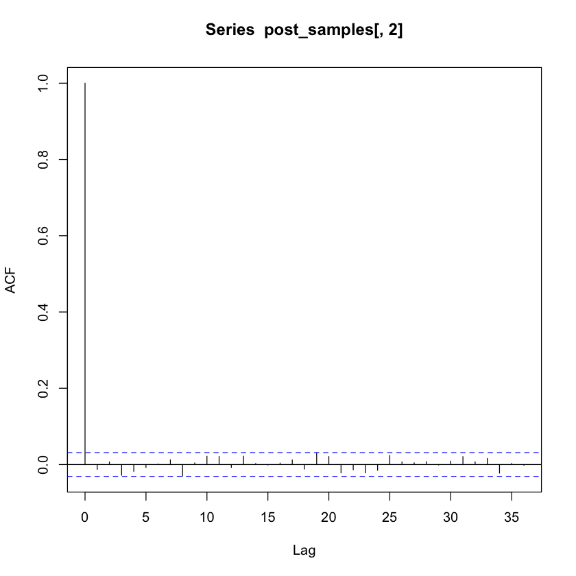
post_samples = extract(samples, "beta")$beta
plot(post_samples[,2])

Informative prior¶

Instead of prior $\beta \sim N(0, 100 \cdot I)$ use $N(0,I)$

samples_i = rstan::stan("logit_informative.stan", 
                         data=crabs_stan)
post_samples_i = extract(samples_i, "beta")$beta

SAMPLING FOR MODEL 'logit_informative' NOW (CHAIN 1).
Chain 1: 
Chain 1: Gradient evaluation took 3.8e-05 seconds
Chain 1: 1000 transitions using 10 leapfrog steps per transition would take 0.38 seconds.
Chain 1: Adjust your expectations accordingly!
Chain 1: 
Chain 1: 
Chain 1: Iteration:    1 / 2000 [  0%]  (Warmup)
Chain 1: Iteration:  200 / 2000 [ 10%]  (Warmup)
Chain 1: Iteration:  400 / 2000 [ 20%]  (Warmup)
Chain 1: Iteration:  600 / 2000 [ 30%]  (Warmup)
Chain 1: Iteration:  800 / 2000 [ 40%]  (Warmup)
Chain 1: Iteration: 1000 / 2000 [ 50%]  (Warmup)
Chain 1: Iteration: 1001 / 2000 [ 50%]  (Sampling)
Chain 1: Iteration: 1200 / 2000 [ 60%]  (Sampling)
Chain 1: Iteration: 1400 / 2000 [ 70%]  (Sampling)
Chain 1: Iteration: 1600 / 2000 [ 80%]  (Sampling)
Chain 1: Iteration: 1800 / 2000 [ 90%]  (Sampling)
Chain 1: Iteration: 2000 / 2000 [100%]  (Sampling)
Chain 1: 
Chain 1:  Elapsed Time: 0.635792 seconds (Warm-up)
Chain 1:                0.358218 seconds (Sampling)
Chain 1:                0.99401 seconds (Total)
Chain 1: 

SAMPLING FOR MODEL 'logit_informative' NOW (CHAIN 2).
Chain 2: 
Chain 2: Gradient evaluation took 1.3e-05 seconds
Chain 2: 1000 transitions using 10 leapfrog steps per transition would take 0.13 seconds.
Chain 2: Adjust your expectations accordingly!
Chain 2: 
Chain 2: 
Chain 2: Iteration:    1 / 2000 [  0%]  (Warmup)
Chain 2: Iteration:  200 / 2000 [ 10%]  (Warmup)
Chain 2: Iteration:  400 / 2000 [ 20%]  (Warmup)
Chain 2: Iteration:  600 / 2000 [ 30%]  (Warmup)
Chain 2: Iteration:  800 / 2000 [ 40%]  (Warmup)
Chain 2: Iteration: 1000 / 2000 [ 50%]  (Warmup)
Chain 2: Iteration: 1001 / 2000 [ 50%]  (Sampling)
Chain 2: Iteration: 1200 / 2000 [ 60%]  (Sampling)
Chain 2: Iteration: 1400 / 2000 [ 70%]  (Sampling)
Chain 2: Iteration: 1600 / 2000 [ 80%]  (Sampling)
Chain 2: Iteration: 1800 / 2000 [ 90%]  (Sampling)
Chain 2: Iteration: 2000 / 2000 [100%]  (Sampling)
Chain 2: 
Chain 2:  Elapsed Time: 0.667282 seconds (Warm-up)
Chain 2:                0.41025 seconds (Sampling)
Chain 2:                1.07753 seconds (Total)
Chain 2: 

SAMPLING FOR MODEL 'logit_informative' NOW (CHAIN 3).
Chain 3: 
Chain 3: Gradient evaluation took 1.7e-05 seconds
Chain 3: 1000 transitions using 10 leapfrog steps per transition would take 0.17 seconds.
Chain 3: Adjust your expectations accordingly!
Chain 3: 
Chain 3: 
Chain 3: Iteration:    1 / 2000 [  0%]  (Warmup)
Chain 3: Iteration:  200 / 2000 [ 10%]  (Warmup)
Chain 3: Iteration:  400 / 2000 [ 20%]  (Warmup)
Chain 3: Iteration:  600 / 2000 [ 30%]  (Warmup)
Chain 3: Iteration:  800 / 2000 [ 40%]  (Warmup)
Chain 3: Iteration: 1000 / 2000 [ 50%]  (Warmup)
Chain 3: Iteration: 1001 / 2000 [ 50%]  (Sampling)
Chain 3: Iteration: 1200 / 2000 [ 60%]  (Sampling)
Chain 3: Iteration: 1400 / 2000 [ 70%]  (Sampling)
Chain 3: Iteration: 1600 / 2000 [ 80%]  (Sampling)
Chain 3: Iteration: 1800 / 2000 [ 90%]  (Sampling)
Chain 3: Iteration: 2000 / 2000 [100%]  (Sampling)
Chain 3: 
Chain 3:  Elapsed Time: 0.663674 seconds (Warm-up)
Chain 3:                0.366902 seconds (Sampling)
Chain 3:                1.03058 seconds (Total)
Chain 3: 

SAMPLING FOR MODEL 'logit_informative' NOW (CHAIN 4).
Chain 4: 
Chain 4: Gradient evaluation took 1.3e-05 seconds
Chain 4: 1000 transitions using 10 leapfrog steps per transition would take 0.13 seconds.
Chain 4: Adjust your expectations accordingly!
Chain 4: 
Chain 4: 
Chain 4: Iteration:    1 / 2000 [  0%]  (Warmup)
Chain 4: Iteration:  200 / 2000 [ 10%]  (Warmup)
Chain 4: Iteration:  400 / 2000 [ 20%]  (Warmup)
Chain 4: Iteration:  600 / 2000 [ 30%]  (Warmup)
Chain 4: Iteration:  800 / 2000 [ 40%]  (Warmup)
Chain 4: Iteration: 1000 / 2000 [ 50%]  (Warmup)
Chain 4: Iteration: 1001 / 2000 [ 50%]  (Sampling)
Chain 4: Iteration: 1200 / 2000 [ 60%]  (Sampling)
Chain 4: Iteration: 1400 / 2000 [ 70%]  (Sampling)
Chain 4: Iteration: 1600 / 2000 [ 80%]  (Sampling)
Chain 4: Iteration: 1800 / 2000 [ 90%]  (Sampling)
Chain 4: Iteration: 2000 / 2000 [100%]  (Sampling)
Chain 4: 
Chain 4:  Elapsed Time: 0.666095 seconds (Warm-up)
Chain 4:                0.425444 seconds (Sampling)
Chain 4:                1.09154 seconds (Total)
Chain 4: 

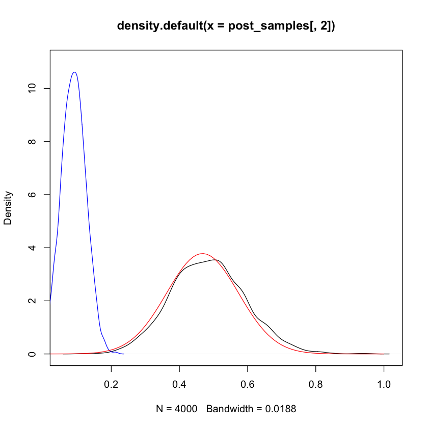
Posterior density for $\beta_{width}$¶

plot(density(post_samples[,2]), ylim=c(0,11))
lines(density(post_samples_i[,2]), col='blue') # with shrinkage
# Bernstein von Mises: using uninformative
# should look Gaussian centered at MLE...
lines(seq(0,1,length=101), 
      dnorm(seq(0,1,length=101), 
            mean=coef(M_crabs)[2], 
            sd=sqrt(vcov(M_crabs)[2,2])), 
      col='red')
mean(post_samples[,2]) # MCMC estimate of posterior mean

0.484950719782206

plot(post_samples[,2], post_samples[,4])
cor(post_samples)

A matrix: 5 × 5 of type dbl
1.00000000	-0.99246293	-0.03396606	0.0546337	-0.01416269
-0.99246293	1.00000000	-0.03624426	-0.1082417	-0.08520037
-0.03396606	-0.03624426	1.00000000	0.2456596	0.46326579
0.05463370	-0.10824175	0.24565961	1.0000000	0.36702285
-0.01416269	-0.08520037	0.46326579	0.3670228	1.00000000

Checking convergence¶

Auto-correlation function of samples¶

acf(post_samples[,2])

Point estimates¶

STAN can find posterior mode / MAP estimator

rstan::optimizing(rstan::stan_model('logit_uninformative.stan'), 
                  data=crabs_stan)
M_crabs$coef

$par

beta[1]: -11.6205948795626
beta[2]: 0.468470895354146
beta[3]: -1.10826097789112
beta[4]: 0.217961072202019
beta[5]: 0.294121635649707

$value

-93.7353861463449

$return_code

0

$theta_tilde

A matrix: 1 × 5 of type dbl
beta[1]	beta[2]	beta[3]	beta[4]	beta[5]
-11.62059	0.4684709	-1.108261	0.2179611	0.2941216

(Intercept): -11.6089904211306
width: 0.467955984822169
colordarker: -1.10612147422922
colorlight: 0.223797656630074
colormedium: 0.296214594694059

STATS 305B

Bayesian methods for GLMs (7.2)¶

Metropolis-Hastings ¶

Gibbs sampling ¶

Gibbs sampler¶

Threshold model¶

Threshold probit model (7.2.6)¶

Gibbs-ish sampler for multivariate truncated Normal¶

STAN ¶

Stan file `logit_uninformative.stan`¶

Informative prior¶

Posterior density for \(\beta_{width}\)¶

Checking convergence¶

Auto-correlation function of samples¶

Point estimates¶

STATS 305B

Bayesian methods for GLMs (7.2)¶

Metropolis-Hastings¶

Gibbs sampling¶

Gibbs sampler¶

Threshold model¶

Threshold probit model (7.2.6)¶

Gibbs-ish sampler for multivariate truncated Normal¶

STAN¶

Stan file logit_uninformative.stan¶

Informative prior¶

Posterior density for \(\beta_{width}\)¶

Checking convergence¶

Auto-correlation function of samples¶

Point estimates¶

Metropolis-Hastings ¶

Gibbs sampling ¶

STAN ¶

Stan file `logit_uninformative.stan`¶