Models for binary outcomes
Data \((X_i, Y_i), 1 \leq i \leq n\).
Examples:
medical: presence or absence of cancer
financial: bankrupt or solvent
industrial: passes a quality control test or not
For \(0-1\) responses we need to model $\(\pi(x_1, \dots, x_p) = P(Y=1|X_1=x_1,\dots, X_p=x_p)\)$
options(repr.plot.width=5, repr.plot.height=4)
Binary outcomes
Likelihood (\(X\) considered fixed or likelihood considered conditional) $\( -\log L(\pi|Y) = \sum_{i=1}^n - Y_i \log\left(\frac{\pi_i}{1-\pi_i}\right) - \log(1 -\pi_i) \)$
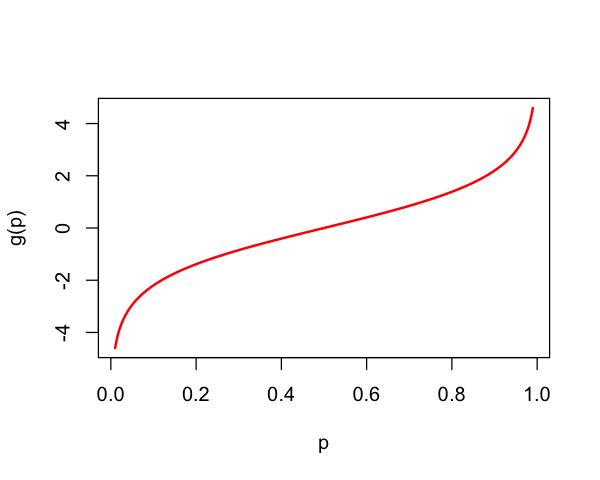
The function $\( \pi \mapsto \log\left(\frac{\pi}{1-\pi}\right) \overset{\text{def}}{=} \text{logit}(\pi) \)$
Logit transform
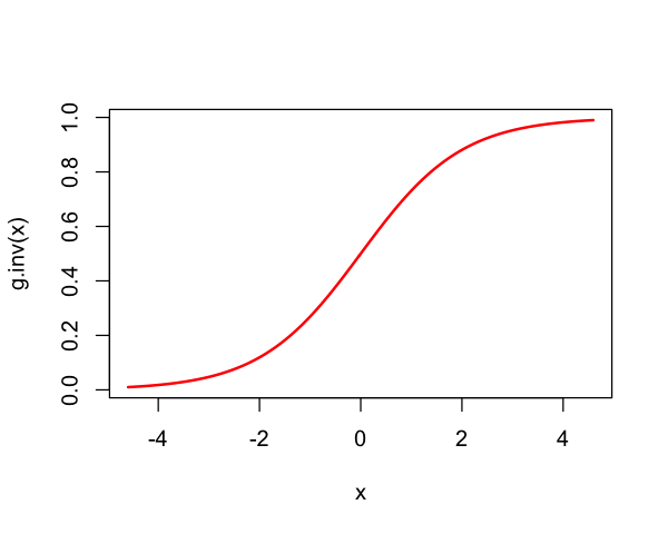
Note $\( \text{logit}\left(\frac{e^{\eta}}{1+e^{\eta}}\right) = \eta. \)\( where \)\( F_{\text{logistic}}(\eta) = \frac{e^{\eta}}{1+e^{\eta}} \)$ is the logistic distribution function.
So, $\( \text{logit} = F_{\text{logistic}}^{-1} \)$
g = function(p) {
  return(log(p / (1 - p)))
}
p = seq(0.01,0.99,length=200)
plot(p, g(p), lwd=2, type='l', col='red')
g.inv <- function(x) {
  return(exp(x) / (1 + exp(x)))
}

x = seq(g(0.01), g(0.99), length=200)
plot(x, g.inv(x), lwd=2, type='l', col='red')
Logistic regression model
Write likelihood in natural parameters
Then,
Logistic regression model: \(\eta_i=X_i^T\beta\) and
Logistic regression
In other words,$\( \text{logit}(\pi(x_1,\dots,x_p)) = x^T\beta. \)$
Negative log-likelihood is convex in \(\beta\) \(\implies\) easy to add regularization penalties (and solve such problems…)
Default in most software for GLMs because(?) \(\eta_i=X_i^T\beta\) (i.e. canonical link)
Logistic regression
How do we know it’s convex?
Negative log-likelihood of saturated model with parameters \(\eta=(\eta_1, \dots, \eta_n)\)
with \(\Lambda_B(\eta)\) the cumulant generating function (CGF) of Bernoulli
For exponential family with sufficient statistic \(W\) and natural parameters \(\eta\)
where \(\mathbb{P}_0\) is the law under \(\eta=0\). In our case
Negative log-likelihood is $\( \eta \mapsto -\eta^TY + \Lambda(\eta) \)$
Logistic regression imposes linear constraint on \(\eta\): \(\eta \in \text{col}(X)\).
Logistic regression
Logistic is “natural” because it is a linear model for natural parameters of Binomial data.
It can appear in other places (c.f. 5.1.5 of Agresti)
Suppose we observe observations from $\( \begin{aligned} Y &\sim \text{Bernoulli}(\pi) \\ X | Y \sim & \begin{cases} N(\mu_0, \Sigma) & Y = 0\\ N(\mu_1, \Sigma) & Y=1 \end{cases} \end{aligned} \)$
Then, logistic model for \(Y|X\) holds.
Another reason this model is popular relates to the odds ratio (c.f. 5.1.4 of Agresti)
If the logistic model is correct along with an assumption about sampling, it is possible to estimate parameters of \(Y|X\) distribution in case-control studies where the actual randomness is \(X|Y\).
This is similar to (2.2.6) of Agresti (Lung Cancer and Smoking) which we discussed earlier.
Interpretation of coefficients: Odds Ratios
Logistic model:
If \(X_j \in \{0, 1\}\) is dichotomous, then odds for group with \(X_j = 1\) are \(e^{\beta_j}\) higher, other parameters being equal.
Rare disease hypothesis
When incidence is rare, \(P(Y=0)\approxeq 1\) no matter what the covariates \(X_j\)’s are.
In this case, odds ratios are almost ratios of probabilities: $\(OR_{X_j} \approxeq \frac{{\mathbb{P}}(Y=1|\dots, X_j=x_j+1, \dots)}{{\mathbb{P}}(Y=1|\dots, X_j=x_j, \dots)}\)$
Hypothetical example: in a lung cancer study, if \(X_j\) is an indicator of smoking or not, a \(\beta_j\) of 5 means for smoking vs. non-smoking means smokers are \(e^5 \approx 150\) times more likely to develop lung cancer
Other (linear) binary models
Suppose there is some latent variable \(T_i | X_i \sim F\) such that
Then,
Example: probit \(F=\Phi\) (dbn of \(N(0,1)\))
Setting $\( \eta_i = \text{logit}(F(X_i^T\beta)) \)\( the likelihood is then \)\( -\log L(\beta|Y) = \sum_{i=1}^n -Y_i \cdot \text{logit}(F(X_i^T\beta)) - \log(1 - F(X_i^T\beta)). \)$
Parameters no longer interpretable in odds ratios but problem can still be convex (e.g. probit)
Modelling probabilities
Note: \(\text{Var}(Y) = \pi ( 1 - \pi) = E(Y) \cdot ( 1- E(Y))\)
The binary nature forces a relation between mean and variance of \(Y\).
This makes logistic regression a Generalized Linear Model, use
glminR.
Horseshoe crabs
library(glmbb) # for `crabs` data
data(crabs)
head(crabs)
| color | spine | width | satell | weight | y | |
|---|---|---|---|---|---|---|
| <fct> | <fct> | <dbl> | <int> | <int> | <int> | |
| 1 | medium | bad | 28.3 | 8 | 3050 | 1 |
| 2 | dark | bad | 22.5 | 0 | 1550 | 0 |
| 3 | light | good | 26.0 | 9 | 2300 | 1 |
| 4 | dark | bad | 24.8 | 0 | 2100 | 0 |
| 5 | dark | bad | 26.0 | 4 | 2600 | 1 |
| 6 | medium | bad | 23.8 | 0 | 2100 | 0 |
width_glm = glm(y ~ width, family=binomial(), data=crabs)
summary(width_glm)
anova(glm(y ~ 1, family=binomial(), data=crabs), width_glm)
c(225.76-194.45, 4.887^2)
Call:
glm(formula = y ~ width, family = binomial(), data = crabs)

Deviance Residuals:
    Min       1Q   Median       3Q      Max
-2.0281  -1.0458   0.5480   0.9066   1.6942

Coefficients:
            Estimate Std. Error z value Pr(>|z|)
(Intercept) -12.3508     2.6287  -4.698 2.62e-06 ***
width         0.4972     0.1017   4.887 1.02e-06 ***
---
Signif. codes:  0 ‘***’ 0.001 ‘**’ 0.01 ‘*’ 0.05 ‘.’ 0.1 ‘ ’ 1

(Dispersion parameter for binomial family taken to be 1)

    Null deviance: 225.76  on 172  degrees of freedom
Residual deviance: 194.45  on 171  degrees of freedom
AIC: 198.45

Number of Fisher Scoring iterations: 4
| Resid. Df | Resid. Dev | Df | Deviance | |
|---|---|---|---|---|
| <dbl> | <dbl> | <dbl> | <dbl> | |
| 1 | 172 | 225.7585 | NA | NA |
| 2 | 171 | 194.4527 | 1 | 31.30586 |
- 31.31
- 23.882769
summary(glm(y ~ width, data=crabs)) # same fit as `lm`
Call:
glm(formula = y ~ width, data = crabs)

Deviance Residuals:
    Min       1Q   Median       3Q      Max
-0.8614  -0.4495   0.1569   0.3674   0.7061

Coefficients:
            Estimate Std. Error t value Pr(>|t|)
(Intercept) -1.76553    0.42136  -4.190 4.46e-05 ***
width        0.09153    0.01597   5.731 4.42e-08 ***
---
Signif. codes:  0 ‘***’ 0.001 ‘**’ 0.01 ‘*’ 0.05 ‘.’ 0.1 ‘ ’ 1

(Dispersion parameter for gaussian family taken to be 0.1951497)

    Null deviance: 39.780  on 172  degrees of freedom
Residual deviance: 33.371  on 171  degrees of freedom
AIC: 212.26

Number of Fisher Scoring iterations: 2
summary(lm(y ~ width, data=crabs))  # dispersion is \hat{\sigma}^2
0.4418^2
Call:
lm(formula = y ~ width, data = crabs)

Residuals:
    Min      1Q  Median      3Q     Max
-0.8614 -0.4495  0.1569  0.3674  0.7061

Coefficients:
            Estimate Std. Error t value Pr(>|t|)
(Intercept) -1.76553    0.42136  -4.190 4.46e-05 ***
width        0.09153    0.01597   5.731 4.42e-08 ***
---
Signif. codes:  0 ‘***’ 0.001 ‘**’ 0.01 ‘*’ 0.05 ‘.’ 0.1 ‘ ’ 1

Residual standard error: 0.4418 on 171 degrees of freedom
Multiple R-squared:  0.1611,	Adjusted R-squared:  0.1562
F-statistic: 32.85 on 1 and 171 DF,  p-value: 4.415e-08
Logistic regression and \(I \times 2\) tables
For \(I \times 2\) tables \(N=(N_{ij})\), set
Under independent rows sampling,
Under Poisson sampling, same result holds if we condition on \(N_{i+}\).
Model
Like a one-way ANOVA regression model
Need some identifiability constraint (
Roften sets one \(\beta\) to 0).Not really using a logistic assumption here – just parameterizing \(\pi_i\) a certain way: model is saturated.
# Table 3.8
absent = c(17066, 14464, 788, 126, 37)
present = c(48, 38, 5, 1, 1)
total = absent + present
scores = c(0, 0.5, 1.5, 4.0, 7.0)
proportion = present / total
alcohol = rbind(absent, present)
chisq.test(alcohol)
Warning message in chisq.test(alcohol):
“Chi-squared approximation may be incorrect”
	Pearson's Chi-squared test

data:  alcohol
X-squared = 12.082, df = 4, p-value = 0.01675
lr_stat = function(data_table) {
    chisq_test = chisq.test(data_table)
    return(2 * sum(data_table * log(data_table / chisq_test$expected)))
}
lr_stat(alcohol)
Warning message in chisq.test(data_table):
“Chi-squared approximation may be incorrect”
alcohol_scores = glm(proportion ~ factor(scores), family=binomial(),
                     weights=total)
summary(alcohol_scores)
Call:
glm(formula = proportion ~ factor(scores), family = binomial(),
    weights = total)

Deviance Residuals:
[1]  0  0  0  0  0

Coefficients:
                  Estimate Std. Error z value Pr(>|z|)
(Intercept)       -5.87364    0.14454 -40.637   <2e-16 ***
factor(scores)0.5 -0.06819    0.21743  -0.314   0.7538
factor(scores)1.5  0.81358    0.47134   1.726   0.0843 .
factor(scores)4    1.03736    1.01431   1.023   0.3064
factor(scores)7    2.26272    1.02368   2.210   0.0271 *
---
Signif. codes:  0 ‘***’ 0.001 ‘**’ 0.01 ‘*’ 0.05 ‘.’ 0.1 ‘ ’ 1

(Dispersion parameter for binomial family taken to be 1)

    Null deviance: 6.2020e+00  on 4  degrees of freedom
Residual deviance: 1.8163e-13  on 0  degrees of freedom
AIC: 28.627

Number of Fisher Scoring iterations: 4
anova(glm(proportion ~ 1, family=binomial(), weights=total),
      glm(proportion ~ factor(scores), family=binomial(), weights=total))
| Resid. Df | Resid. Dev | Df | Deviance | |
|---|---|---|---|---|
| <dbl> | <dbl> | <dbl> | <dbl> | |
| 1 | 4 | 6.201998e+00 | NA | NA |
| 2 | 0 | 1.816325e-13 | 4 | 6.201998 |
A 1 df test
In this case,
scoresis ordered, so we might fit model $\( \text{logit}(\pi_i) = \alpha + \beta \cdot \text{scores}_i. \)$Perhaps more power because direction of deviation from null is specified.
summary(glm(proportion ~ scores, family=binomial(), weights=total))
Call:
glm(formula = proportion ~ scores, family = binomial(), weights = total)

Deviance Residuals:
      1        2        3        4        5
 0.5921  -0.8801   0.8865  -0.1449   0.1291

Coefficients:
            Estimate Std. Error z value Pr(>|z|)
(Intercept)  -5.9605     0.1154 -51.637   <2e-16 ***
scores        0.3166     0.1254   2.523   0.0116 *
---
Signif. codes:  0 ‘***’ 0.001 ‘**’ 0.01 ‘*’ 0.05 ‘.’ 0.1 ‘ ’ 1

(Dispersion parameter for binomial family taken to be 1)

    Null deviance: 6.2020  on 4  degrees of freedom
Residual deviance: 1.9487  on 3  degrees of freedom
AIC: 24.576

Number of Fisher Scoring iterations: 4
anova(glm(proportion ~ 1, family=binomial(), weights=total),
      glm(proportion ~ scores, family=binomial(), weights=total)) # LR test
data.frame(df.1=pchisq(4.25, 1, lower.tail=FALSE),
           df.4=pchisq(6.2, 4, lower.tail=FALSE))
| Resid. Df | Resid. Dev | Df | Deviance | |
|---|---|---|---|---|
| <dbl> | <dbl> | <dbl> | <dbl> | |
| 1 | 4 | 6.201998 | NA | NA |
| 2 | 3 | 1.948721 | 1 | 4.253277 |
| df.1 | df.4 |
|---|---|
| <dbl> | <dbl> |
| 0.03925033 | 0.1847017 |
Deviance
Instead of sum of squares, logistic regression uses deviance:
Defined as
where \(\pi\) is a location estimator for \(Y\) with \(\hat{\pi}_S\) the saturated fit (i.e. no contraints on \(\pi\)’s).
For Binomial data \(Y_i \sim \text{Binom}({\tt total}_i,\pi_i)\)
If \(Y\) is a binary vector, with mean vector \(\pi\) then
If \(Y_i \sim \text{Binom}({\tt total}_i,\pi_i)\) then
with \(\hat{\pi}_{S,i} = Y_i / {\tt total}_i\) is the MLE under the saturated model.
Fit using
weights=totalinglm.
Deviance for logistic regression
For any binary regression model, the deviance is:
For the logistic model, the RHS is:
The logistic model is special in that \(\text{logit}(\pi_i(\beta))=X_i^T\beta\).
Fitting the logistic model
Derivatives of log-likelihood
Let \(Y \in \{0,1\}^n, X \in \mathbb{R}^{n \times p}\).
Gradient / Score
Hessian
Above,
Derivatives related to moments as this is an exponential family (conditional on \(X\)) with natural parameter \(\beta\), sufficient statistic \(X^TY\) and cumulant generating function
Newton-Raphson
Given initial \(\hat{\beta}^{(0)}\)
Until convergence $\( \hat{\beta}^{(i+1)} = \hat{\beta}^{(i)} - (X^T W_{\hat{\beta}^{(i)}}(X)X)^{-1}X^T(Y - \pi_{\hat{\beta}^{(i)}}(X)) \)$
Inference
Suppose model is true, with true parameter \(\beta^*\). Then, $\( E_{\beta^*}[X^T(Y - \pi_{\beta^*}(X))] = 0 \)$
Taylor series $\( \pi_{\hat{\beta}}(X) \approx \pi_{\beta^*}(X) + W_{\beta^*}(X) X(\hat{\beta}-\beta^*) \)$
How big is remainder?
Inference
Stationarity conditions then read $\( X^T(Y - E_{\beta^*}[Y|X]) \approx X^TW_{\beta^*}(X) X(\hat{\beta}-\beta^*) \)$
Or, $\( \begin{aligned} \hat{\beta}-\beta^* &\approx \left(X^TW_{\beta^*}(X) X\right)^{-1}X^T(Y - E_{\beta^*}[Y|X]) \\ &= (X^TW_{\beta^*}(X)X)^{-1}X^T(Y-\pi_{\beta^*}(X)) \end{aligned} \)$
Implies $\( \begin{aligned} \text{Var}_{\beta^*}(\hat{\beta}-\beta^*) &\approx \left(X^TW_{\beta}^*(X) X\right)^{-1} \text{Var}_{\beta^*}\left(X^T(Y - \pi_{\beta^*}(X))\right) \left(X^TW_{\beta^*}(X) X\right)^{-1} \\ &\approx \left(X^T W_{\beta^*}(X) X\right)^{-1} \\ \end{aligned} \)$ (Last line assumes the model is true.)
Leads to
(Plugin estimator of variance appeals to Slutsky, consistency of \(\hat{\beta}\).)
Where do we really use the model?
Under the logistic model$\( \begin{aligned} \text{Var}_{\beta^*}(X^T(Y-\pi_{\beta}^*(X)) & \approx X^TW_{\beta^*}(X)X. \end{aligned} \)$
Really just using the standard asymptotic distribution of the MLE:
For logistic regression, note that (conditional on \(X\)) $\( E_{\beta^*}[\nabla^2 (-\log L(\beta^*|Y))] = \nabla^2 (-\log L(\beta^*|Y)). \)$
center = coef(width_glm)['width']
SE = sqrt(vcov(width_glm)['width', 'width'])
U = center + SE * qnorm(0.975)
L = center + SE * qnorm(0.025)
data.frame(L, center, U)
| L | center | U | |
|---|---|---|---|
| <dbl> | <dbl> | <dbl> | |
| width | 0.2978326 | 0.4972306 | 0.6966286 |
These are slightly different from what R will give you if you ask it for
confidence intervals:
confint(width_glm)
Waiting for profiling to be done...
| 2.5 % | 97.5 % | |
|---|---|---|
| (Intercept) | -17.8100090 | -7.4572470 |
| width | 0.3083806 | 0.7090167 |
What is logistic regression even estimating?
Before appealing to general properties of MLE, we had only really used the assumption the model was true once.
What can we say if the model is not true?
Suppose \((Y_i,X_i) \overset{IID}{\sim} F, 1 \leq i \leq n\).
Define the population parameter \(\beta^*=\beta^*(F)\) by $\( E_F[X(Y - \pi_{\beta^*(F)}(X))] = 0. \)$
This is minimizer of
Taylor expansion yields
Note that (under conditions…)
Implies $\( \hat{\beta}-\beta^*(F) \overset{D}{\to} N(0, n^{-1} Q(F)^{-1}\Sigma(F)Q(F)^{-1}). \)$
Variance above has so-called sandwich form.
Applying Slutsky $\( \hat{\beta}-\beta^*(F) \approx N\left(0, (X^TW_{\hat{\beta}}(X) X)^{-1} (n\Sigma(F)) (X^TW_{\hat{\beta}}(X) X)^{-1}\right) \)$
We know everything in the approximation above (or can estimate it) except \(\Sigma(F)\)
Covariance \(\Sigma(F)\) can be estimated, say, by bootstrap or sandwich estimator. (Approachable description by D. Freedman here).
Alternatively, entire logistic regression could be bootstrapped.
Testing in logistic regression
What about comparing full and reduced model?
For a model \({\cal M}\), \(DEV({\cal M})\) replaces \(SSE({\cal M})\).
In least squares regression, we use
This is replaced with (when model true)
These tests assume model \({\cal M}_F\) is correctly specified. Otherwise, Wald-type test with sandwich or other covariance estimate would have to be used.
Deviance tests do not agree numerically with Wald tests even when model is correct. Both are often used. Wald can fail!
bigger_glm = glm(y ~ width + weight, data=crabs, family=binomial())
anova(width_glm, bigger_glm)
| Resid. Df | Resid. Dev | Df | Deviance | |
|---|---|---|---|---|
| <dbl> | <dbl> | <dbl> | <dbl> | |
| 1 | 171 | 194.4527 | NA | NA |
| 2 | 170 | 192.8919 | 1 | 1.560777 |
We should compare this difference in deviance with a \(\chi^2_1\) random variable.
1 - pchisq(1.56,1)
Let’s compare this with the Wald test:
summary(bigger_glm)
Call:
glm(formula = y ~ width + weight, family = binomial(), data = crabs)

Deviance Residuals:
    Min       1Q   Median       3Q      Max
-2.1127  -1.0344   0.5304   0.9006   1.7207

Coefficients:
              Estimate Std. Error z value Pr(>|z|)
(Intercept) -9.3547261  3.5280465  -2.652  0.00801 **
width        0.3067892  0.1819473   1.686  0.09177 .
weight       0.0008338  0.0006716   1.241  0.21445
---
Signif. codes:  0 ‘***’ 0.001 ‘**’ 0.01 ‘*’ 0.05 ‘.’ 0.1 ‘ ’ 1

(Dispersion parameter for binomial family taken to be 1)

    Null deviance: 225.76  on 172  degrees of freedom
Residual deviance: 192.89  on 170  degrees of freedom
AIC: 198.89

Number of Fisher Scoring iterations: 4