Loglinear models (Chs. 9 & 10)
Models for contingency tables
Estimation via pseudo-likelihood.
Two-way tables
\(N_{ij} \sim \text{Poisson}(\mu_{ij})\), \(1 \leq i \leq I, 1 \leq j \leq J\)
Independence model $\( \log(\mu_{ij}) = \lambda + \lambda_i^X + \lambda_j^Y \)$
Saturated model $\( \log(\mu_{ij}) = \lambda + \lambda_i^X + \lambda_j^Y + \lambda_{ij}^{XY} \)$
Model for joint law
Can be thought of as drawing a Poisson number of samples from some joint distribution for \((X,Y)\):
Saturated model is overparametrized, typical constraints (using baseline categories)
Form of regression function implies conditional independencies when using log-linear model.
Three way tables (9.3)
Saturated
Homogeneous association model: \(\lambda^{XYZ}_{ijk} \equiv 0\) (more generally, no 3-way or higher interactions)
Mutual independence
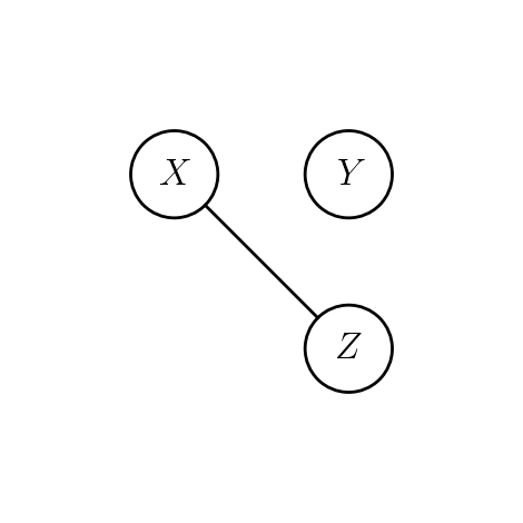
Joint independence: \(Y\) independent of \((X,Z)\)
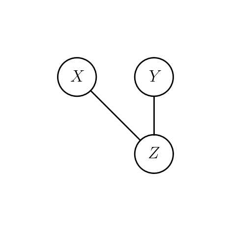
Conditional independence of \(Y\) and \(X\) given \(Z\)
Test of conditional independence
# Table 9.1 of Agresti
library(vcdExtra) # for `DaytonSurvey` data
data(DaytonSurvey)
Dayton.aggregated = aggregate(Freq ~ cigarette + alcohol + marijuana,
                              data=DaytonSurvey, FUN=sum)
Dayton.aggregated
Loading required package: vcd
Loading required package: grid
Loading required package: gnm
| cigarette | alcohol | marijuana | Freq |
|---|---|---|---|
| <fct> | <fct> | <fct> | <dbl> |
| Yes | Yes | Yes | 911 |
| No | Yes | Yes | 44 |
| Yes | No | Yes | 3 |
| No | No | Yes | 2 |
| Yes | Yes | No | 538 |
| No | Yes | No | 456 |
| Yes | No | No | 43 |
| No | No | No | 279 |
full.model = glm(Freq ~ .^2, data=Dayton.aggregated, family=poisson)  # homogeneous association: only up to 2way interactions
summary(full.model)
Call:
glm(formula = Freq ~ .^2, family = poisson, data = Dayton.aggregated)

Deviance Residuals:
       1         2         3         4         5         6         7         8
 0.02044  -0.09256  -0.33428   0.49134  -0.02658   0.02890   0.09452  -0.03690

Coefficients:
                        Estimate Std. Error z value Pr(>|z|)
(Intercept)              6.81387    0.03313 205.699  < 2e-16 ***
cigaretteNo             -3.01575    0.15162 -19.891  < 2e-16 ***
alcoholNo               -5.52827    0.45221 -12.225  < 2e-16 ***
marijuanaNo             -0.52486    0.05428  -9.669  < 2e-16 ***
cigaretteNo:alcoholNo    2.05453    0.17406  11.803  < 2e-16 ***
cigaretteNo:marijuanaNo  2.84789    0.16384  17.382  < 2e-16 ***
alcoholNo:marijuanaNo    2.98601    0.46468   6.426 1.31e-10 ***
---
Signif. codes:  0 ‘***’ 0.001 ‘**’ 0.01 ‘*’ 0.05 ‘.’ 0.1 ‘ ’ 1

(Dispersion parameter for poisson family taken to be 1)

    Null deviance: 2851.46098  on 7  degrees of freedom
Residual deviance:    0.37399  on 1  degrees of freedom
AIC: 63.417

Number of Fisher Scoring iterations: 4
reduced.model = glm(Freq ~ alcohol + marijuana + cigarette +
                    alcohol:marijuana +
                    cigarette:marijuana,
                    data=Dayton.aggregated, family=poisson)
summary(reduced.model)
Call:
glm(formula = Freq ~ alcohol + marijuana + cigarette + alcohol:marijuana +
    cigarette:marijuana, family = poisson, data = Dayton.aggregated)

Deviance Residuals:
      1        2        3        4        5        6        7        8
 0.0584  -0.2619  -0.8663   2.2287   4.5702  -4.3441  -9.7716   6.8353

Coefficients:
                        Estimate Std. Error z value Pr(>|z|)
(Intercept)              6.81261    0.03316 205.450   <2e-16 ***
alcoholNo               -5.25227    0.44837 -11.714   <2e-16 ***
marijuanaNo             -0.72847    0.05538 -13.154   <2e-16 ***
cigaretteNo             -2.98919    0.15111 -19.782   <2e-16 ***
alcoholNo:marijuanaNo    4.12509    0.45294   9.107   <2e-16 ***
marijuanaNo:cigaretteNo  3.22431    0.16098  20.029   <2e-16 ***
---
Signif. codes:  0 ‘***’ 0.001 ‘**’ 0.01 ‘*’ 0.05 ‘.’ 0.1 ‘ ’ 1

(Dispersion parameter for poisson family taken to be 1)

    Null deviance: 2851.46  on 7  degrees of freedom
Residual deviance:  187.75  on 2  degrees of freedom
AIC: 248.8

Number of Fisher Scoring iterations: 5
anova(reduced.model, full.model) # null: conditional independence of alcohol & cigarette | marijuana
| Resid. Df | Resid. Dev | Df | Deviance | |
|---|---|---|---|---|
| <dbl> | <dbl> | <dbl> | <dbl> | |
| 1 | 2 | 187.7543029 | NA | NA |
| 2 | 1 | 0.3739859 | 1 | 187.3803 |
Homogeneous association
If we fix \(Z=k\), then the dependence of \((X,Y)|Z=k\) can be described by local odds ratios of 2x2 table for \(X\in \{i,i+1\}\) and \(Y\in \{j,j+1\}\)
Under homogeneous association, these do not depend on \(k\)
Similarly for \(\theta_{(i)jk}\) and \(\theta_{i(j)k}\).
Higher dimensional tables (9.4)
Homogeneous association model: no three way interactions
In homogeneous association model, conditional independencies can be read off an undirected graph on vertices \(\{X,Y,Z,W\}\).
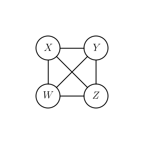
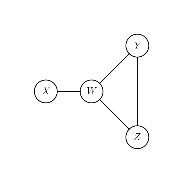
Homogeneous model with this graph has same conditional independencies as \((XW, WYZ)\).
\(\implies\) conditional independencies are not going to tell us whether there are any 3-way interactions or not.
\(W\) is conditionally independent of \(Y\) given \((X,Z)\).
\(X\) is conditionally independent of \(Z\) given \((W,Y)\).
Model: \(\lambda^{XZ}_{ik} \equiv 0, \lambda^{YW}_{jl} \equiv 0\).
Generally, for vertex \(v\) set \(N(v)\) to be its neighbors in the graph \(G=(E,V)\).
The conditional independencies: \(v\) is independent of \((\{v\} \cup N(v))^c\) given \(N(v)\).

Connection with logistic regression (9.5)
For simplicity let’s assume each of \((X,Y,Z,W)\) is binary.
In complete graph
A logistic regression model with Binomial outcome \(Y_{ikl}\) and 3-column design matrix.
Number of rows is total count in the \(2x2x2x2\) table.
In smaller graph
Features for the logistic regression model for \(Y\) determined by \(N(Y)\).
Design matrix has 2 columns plus intercept.
Logistic regression model for \(Y\) allows us to estimate:
\(\lambda^Y_1 - \lambda^Y_0\)
\(\lambda^{XY}_{11} - \lambda^{XY}_{10} - \lambda^{XY}_{01} + \lambda^{XY}_{00}\)
\(\lambda^{YW}_{11} - \lambda^{YW}_{01} - \lambda^{YW}_{10} + \lambda^{YW}_{00}\)
Logistic regression model for \(X\) allows us to estimate:
\(\lambda^X_1 - \lambda^X_0\)
\(\lambda^{XY}_{11} - \lambda^{XY}_{01} - \lambda^{XY}_{10} + \lambda^{XY}_{00}\)
\(\lambda^{XW}_{11} - \lambda^{XW}_{01} - \lambda^{XW}_{10} + \lambda^{XW}_{00}\)
Non-binary data
Categorical models become baseline multinomial logits.
We estimate matrices of parameters – more complicated notation, conceptually the same.
How to estimate? (Especially if number of variables grow)
Usual default constraints would set anything with a 0 in subscript to 0…
With these constraints, we get two estimates for \(\lambda^{XY}_{11} - \lambda^{XY}_{10} - \lambda^{XY}_{01} + \lambda^{XY}_{00}\) (equal to \(\lambda^{XY}_{11}\) under defaults), one from each logistic regression.
Actually three – one comes from the loglinear model.
Which interactions to include? (To be revisited later.)
Pseudolikelihood
Each of \(X,Y,Z,W\) has a corresponding logistic regression model formed by conditioning on its neighbours.
The pseudo-likelihood for parameters \(\Lambda = (\lambda, \lambda^X_i, \lambda^Y_j, \dots)\) is
References:
Several more in between…
Exact likelihood
Suppose now we have vertices \(V = \{X_1, \dots, X_k\}\) where each \(X_i \in \{0,1\}\) and graph \(G=(E,V)\)
For binary data and usual constraints on parameters each vertex in \(V\) gets one parameter and each edge gets one parameter. One parameter \(\gamma\) for overall intensity.
Edge / vertex parameters can be represented by symmetric matrix \(\Theta\) with \(\Theta_{ij} \neq 0 \iff (i,j) \in E\).
Likelihood (with a little work, assuming we observe full table)
where
Set \(B \in \{0,1\}^{\text{sum}(N) \times V}\). Then
Normalizing constant is expensive to compute for moderate \(k\).
Pseudolikelihood
Pseudo-likelihood is a sum of \(k\) different logistic regression log-likelihoods.
The parameters in the log-likelihoods are functions of \((\gamma, \Theta)\) – pseudolikelihood ties them all together.
Normalizing constant is simple.
Fit is very easy.
Downside
Since this is not a likelihood, cannot appeal to LR tests, Fisher information.
Bootstrap likely applicable.
Non-binary data
If a variable \(X_i\) is not binary, then its pseudo-likelihood is baseline multinomial logit log-likelihood.
In this case, \(\Theta\) is not a matrix, every edge is represented by potentially a matrix of parameters.
Selecting interactions (i.e. edges)
Pseudolikelihood for Ising model
Besag’s original motivation was for inference in models similar to an Ising model and other models of spatial statistics.
Given graph \(G=(V,E)\) and a single observation \(X \in \{0,1\}^V\), we want to estimate parameters in a model
This is an exponential family:
Sufficient statistics: \(\left(\sum_{i \in V} X_i, \sum_{(i,j) \in E}X_i X_j \right)\)
Natural parameters: \((\alpha, \beta)\)
Reference measure: counting measure on \(\{0,1\}^V\).
Contribution of a vertex
Terms in the pseudolikelihood are
Log-pseudolikelihood, summing over \(i\) is $\( \sum_{i \in V} \left(\alpha \cdot X_i + \beta \left(\sum_{j \in N(i)} X_iX_j\right) \right) - \log\left(1 + \exp\left(\alpha + \beta \sum_{j \in N(i)} X_j\right) \right) \)$
Differentiate w.r.t. \(\alpha\) $\( \sum_{i \in V} \left[X_i - \frac{\exp\left(\alpha + \beta \sum_{j \in N(i)} X_j \right)}{1 + \exp\left(\alpha + \beta \sum_{j \in N(i)} X_j \right)} \right] \)$
Computing expectations at true \((\alpha^*,\beta^*)\):
At pseudo-MLE we set this equal to $\( 0= E_{(\alpha^*,\beta^*)} \left[\sum_{i \in V} \left[E_{(\alpha^*,\beta^*)}[X_i|X_{N(i)}] - \frac{\exp\left(\alpha^* + \beta^* \sum_{j \in N(i)} X_j \right)}{1 + \exp\left(\alpha^* + \beta^* \sum_{j \in N(i)} X_j \right)} \right] \right] \)$
Pseudo-likelihood is an estimating equation…
Implications for Gibbs sampling
Suppose we want to sample from \(P_{(\alpha,\beta)}\).
Distribution \(X_i | X_{-i}\) is the same as \(X_i | X_{N(i)}\).
Posterior densities used for Gibbs sampling correspond to pseudo-likelihoods times priors
Other uses of pseudolikelihood
The “pieces” of pseudolikelihood are conditional likelihoods.
These conditional likelihoods are sometimes useful themselves following general principle of eliminating nuisance parameters.
In the homogeneous association model conditioning on all neighbours eliminate all nuisance parameters for all variables outside of \(\{v\} \cup N(v)\).
OLS regression
Consider the usual Gaussian regression model with \((\beta,\sigma^2)\) unknown
An exponential family:
Sufficient statistic \((X^TY, \|Y\|^2_2)\).
Natural parameters \(\left(\beta / \sigma^2, -\frac{1}{2\sigma^2}\right)\)
Reference measure: \(dY\).
Consider the law $\(P_{(\beta, \sigma^2)}\left(\|Y\|^2_2 \bigl \vert X^TY\right).\)$
Not hard to see that this law is \(\|(I-H)Y\|^2_2 + \|HY\|^2_2\) where \(HY\) is measurable w.r.t. \(X^TY\).
Conditional likelihood for \(\sigma^2\) is based on \(P_{(\beta,\sigma^2)}(\|(I-H)Y\|^2_2)\) – a \(\chi^2_{n-p}\) likelihood.
Maximum (conditional) likelihood estimator is the usual unbiased estimate of \(\sigma^2\) not the biased MLE. This conditional likelihood estimator is better than the MLE!
This phenomenon has a life of its own in mixed effects model: REML (Residual Maximum Likelihood) (though elimination of nuisance parameter is not always justified by conditioning).
Continuous variables
We saw with binary data marginal homogeneity yields a model with likelihood
Suppose data are continuous but marginally homogeneous.
A few choices yields Gaussian: \(X_s \sim N(0,\Sigma), 1 \leq s \leq n\)
Above
Setting \(\Theta=\Sigma^{-1}\) yields
Unlike binary case normalizing constant is explicit.
Selecting edges: graphical LASSO
This uses true likelihood because normalizing constant is known.