Grouped goodness of fit tests (5.2.5)
library(glmbb) # for `crabs` data
data(crabs)
width_glm = glm(y ~ width, family=binomial(), data=crabs)
Is the logistic model a good fit?
library(dplyr)
crabs$groups = cut(crabs$width, breaks=c(0, seq(23.25, 29.25, by=1), max(crabs$width)))
crabs$fits = fitted(width_glm)
results = crabs %>%
          group_by(groups) %>%
          summarize(N=n(), numY = sum(y), numN = N - numY,
                    fittedY=sum(fits), fittedN=N-fittedY)
results
Attaching package: ‘dplyr’
The following objects are masked from ‘package:stats’:

    filter, lag
The following objects are masked from ‘package:base’:

    intersect, setdiff, setequal, union
`summarise()` ungrouping output (override with `.groups` argument)
| groups | N | numY | numN | fittedY | fittedN |
|---|---|---|---|---|---|
| <fct> | <int> | <int> | <int> | <dbl> | <dbl> |
| (0,23.2] | 14 | 5 | 9 | 3.635428 | 10.3645724 |
| (23.2,24.2] | 14 | 4 | 10 | 5.305988 | 8.6940124 |
| (24.2,25.2] | 28 | 17 | 11 | 13.777624 | 14.2223757 |
| (25.2,26.2] | 39 | 21 | 18 | 24.227680 | 14.7723199 |
| (26.2,27.2] | 22 | 15 | 7 | 15.937800 | 6.0621999 |
| (27.2,28.2] | 24 | 20 | 4 | 19.383348 | 4.6166516 |
| (28.2,29.2] | 18 | 15 | 3 | 15.650178 | 2.3498224 |
| (29.2,33.5] | 14 | 14 | 0 | 13.081954 | 0.9180457 |
G2 = 2 * (sum(results$numY * log(results$numY / results$fittedY)) +
          sum(results$numN * log((results$numN + 1.e-10) / results$fittedN)))
c(G2, pchisq(G2, 8 - 2, lower.tail=FALSE)) # why df=6?
- 6.17936230993838
- 0.403400865096638
X2 = (sum((results$numY - results$fittedY)^2 / results$fittedY) +
      sum((results$numN - results$fittedN)^2 / results$fittedN))
c(X2, pchisq(X2, 8 - 2, lower.tail=FALSE))
- 5.32009943957515
- 0.503461006750787
Hosmer-Lemeshow
Alternative “partition”: partition cases based on \(\hat{\pi}\).
Rank \(\hat{\pi}\) into \(g\) groups.
Compute Pearson’s \(X^2\) as above.
library(ResourceSelection)
hoslem.test(crabs$y, crabs$fits, g=10)
ResourceSelection 0.3-5 2019-07-22
	Hosmer and Lemeshow goodness of fit (GOF) test

data:  crabs$y, crabs$fits
X-squared = 4.3855, df = 8, p-value = 0.8208
Diagnostics in logistic regression (6.2)
If we have grouped data (i.e. a fixed number of possible covariate values) we can use a \(G^2\) or \(X^2\) test as a goodness of fit.
Without groups, we might make groups by partitioning the feature space appropriately.
Residuals
Pearson residual $\( e_i = \frac{Y_i - \hat{\pi}_i}{\sqrt{\hat{\pi}_i(1-\hat{\pi}_i)}} \)$
Used to form Pearson’s \(X^2\) (we’ll see general form for GLMs later) $\( X^2 = \sum_{i=1}^n e_i^2. \)$
Residuals
Deviance residual: write deviance as $\( DEV(\hat{\pi}|Y) = \sum_{i=1}^n DEV(\hat{\pi}_i|Y_i) \)\( then the deviance residuals are \)\( \text{sign}(Y_i-\hat{\pi}_i) \cdot \sqrt{DEV(\hat{\pi}_i|Y_i)} \)$
Hat matrix and leverage
As in OLS regression, residuals have smaller variance than the true errors. (What are the true errors?)
In OLS regression, this is remedied by standardizing $\( r_i = \frac{Y_i - \hat{Y}_i} {\sqrt{R_{ii}}} \)\( where \)R=I-H\( is the residual forming matrix and \)\( H = X(X^TX)^{-1}X^T \)$ is the hat matrix.
What is analog of \(H\) in logistic regression?
Hat matrix and leverage
Recall $\( \begin{aligned} \hat{\beta}-\beta^* &\approx (X^TW_{\beta^*}X)^{-1}X^T(Y-\pi_{\beta^*}(X)) \\ &= (X^TW_{\beta^*}X)^{-1}X^TW^{1/2}_{\beta^*}R_{\beta^*}(X,Y) \\ \end{aligned} \)$
Above, $\( R_{\beta^*}(X,Y) = W_{\beta^*}^{-1/2}(Y-\pi_{\beta^*}(X)) \)$ has independent entries, each with variance 1 (assuming model is correctly specified).
\(Z_{\beta^*}(X,Y)\) are essentially the (population) Pearson residuals…
Hat matrix and leverage
We see \(\hat{\beta}\) is essentially OLS estimator with design \(W_{\beta^*}^{1/2}(X)X\) and errors \(R_{\beta^*}(X,Y)\) (This is basically the IRLS viewpoint)
In this OLS model, the appropriate hat matrix is
approximated by
Standardized residuals
Given “correct” hat matrix, leads to standardized residual
Residuals and leverage can be used in similar ways as in OLS:
Detect outliers. (Are they normal? Probably not. Grouped data has a chance.)
Check regression specification.
library(car)
outlierTest(width_glm)
Loading required package: carData
Attaching package: ‘car’
The following object is masked from ‘package:dplyr’:

    recode
No Studentized residuals with Bonferroni p < 0.05
Largest |rstudent|:
   rstudent unadjusted p-value Bonferroni p
94 -2.05045           0.040321           NA
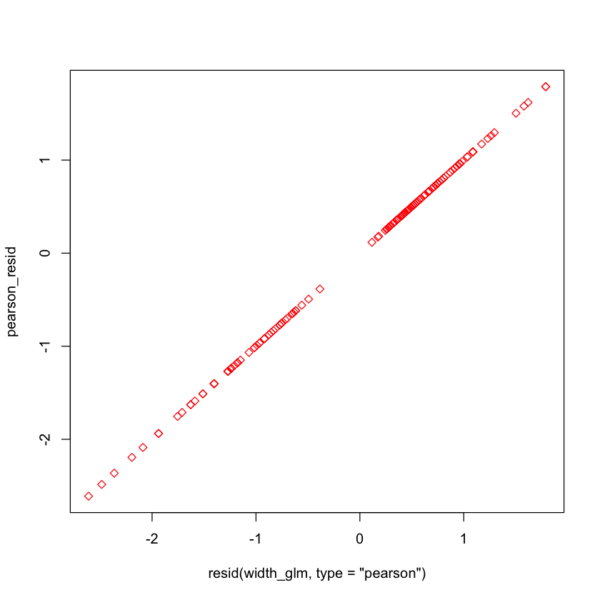
pearson_resid = (crabs$y - crabs$fits) / sqrt(crabs$fits * (1 - crabs$fits))
plot(resid(width_glm, type='pearson'), pearson_resid, pch=23, col='red')
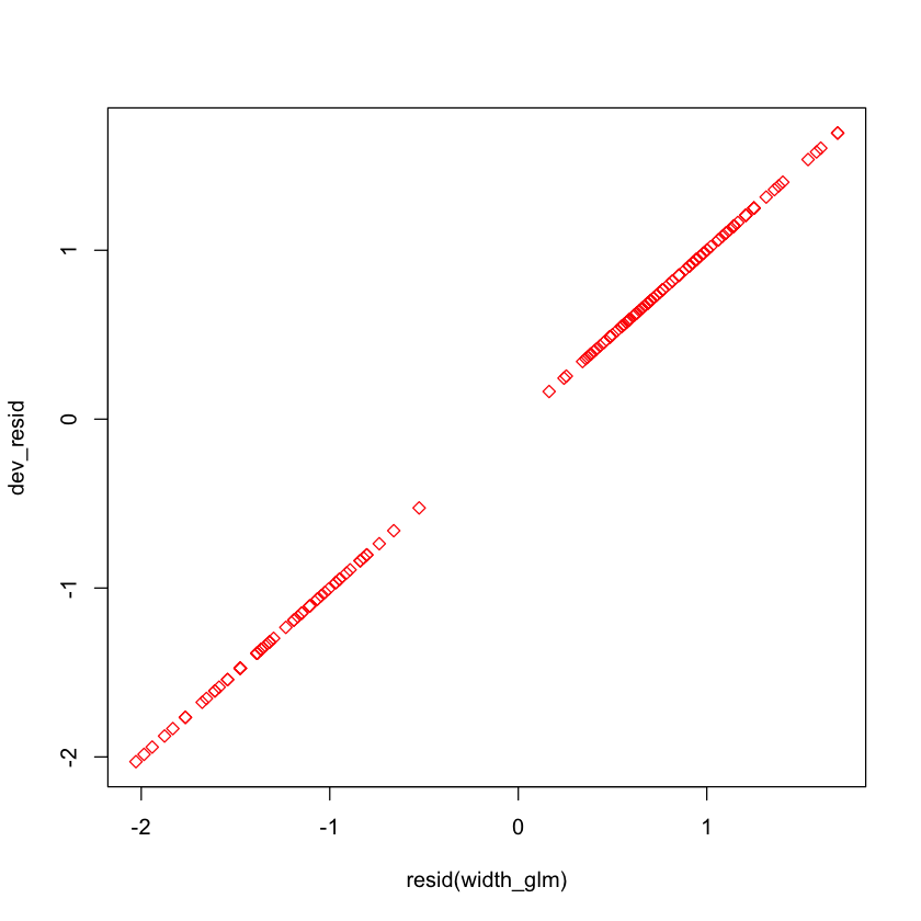
dev_resid = sign(crabs$y - crabs$fits) *
     sqrt(- 2 * (crabs$y * log(crabs$fits) + (1 - crabs$y) * log(1 - crabs$fits)))
plot(resid(width_glm), dev_resid, pch=23, col='red')
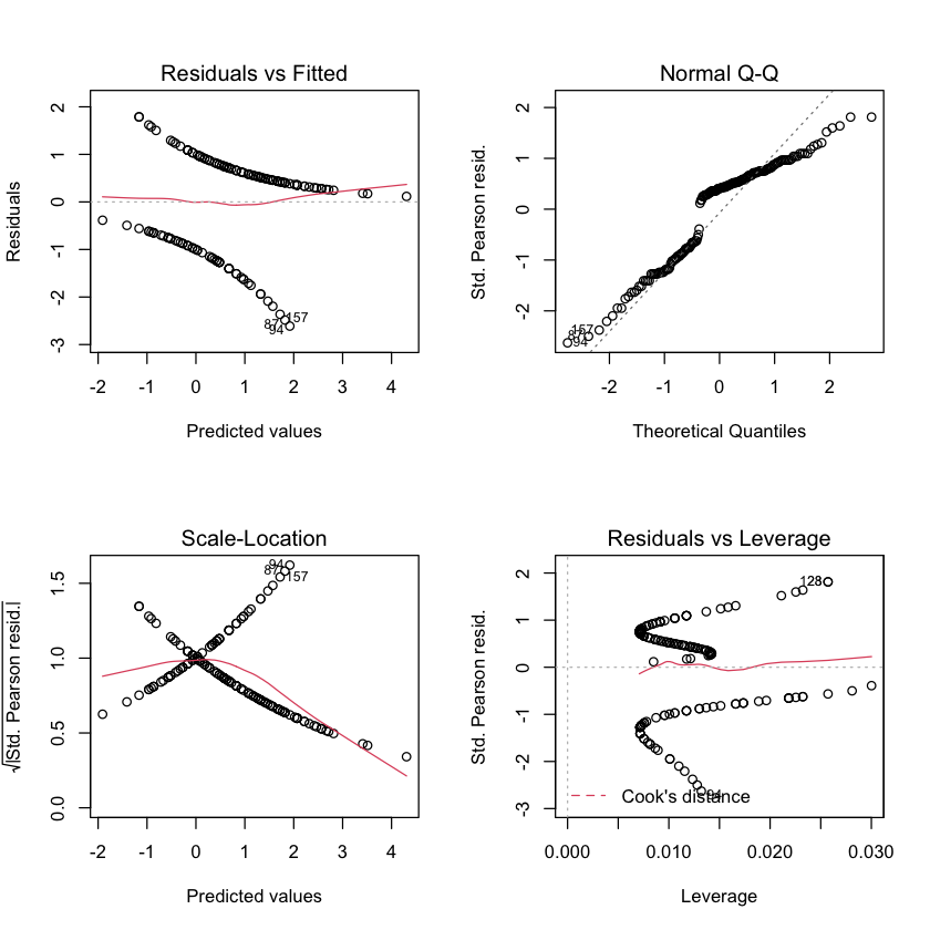
par(mfrow=c(2,2))
plot(width_glm)
Analog of \(R^2\) (6.3)
In OLS regression, a common summary is $\( R^2 = 1 - \frac{SSE}{SST} = \frac{SST-SSE}{SST} \)$
Analog for logistic regression is McFadden’s \(R^2\) $\( \frac{DEV(M_0) - DEV(M)}{DEV(M_0)} \)$
anova(width_glm)
c((225.76 - 194.45) / 225.76,
  1 - width_glm$deviance / width_glm$null.deviance)
| Df | Deviance | Resid. Df | Resid. Dev | |
|---|---|---|---|---|
| <int> | <dbl> | <int> | <dbl> | |
| NULL | NA | NA | 172 | 225.7585 |
| width | 1 | 31.30586 | 171 | 194.4527 |
- 0.138687101346563
- 0.138669667388724
Influence measures
library(car)
head(influence.measures(width_glm)$infmat)
| dfb.1_ | dfb.wdth | dffit | cov.r | cook.d | hat | |
|---|---|---|---|---|---|---|
| 1 | -0.047610662 | 0.04996645 | 0.06040203 | 1.020937 | 0.001132128 | 0.012344511 |
| 2 | -0.104054950 | 0.10079960 | -0.11366303 | 1.032553 | 0.004233338 | 0.025717205 |
| 3 | -0.004535225 | 0.00948021 | 0.07499977 | 1.009632 | 0.002017305 | 0.007084208 |
| 4 | -0.061618758 | 0.05535952 | -0.11116748 | 1.007620 | 0.005034932 | 0.010062537 |
| 5 | -0.004535225 | 0.00948021 | 0.07499977 | 1.009632 | 0.002017305 | 0.007084208 |
| 6 | -0.094872323 | 0.08993360 | -0.11878283 | 1.018836 | 0.005119353 | 0.016600380 |
Confusion matrix
Suppose classification rule is $\( \hat{y}(x) = \begin{cases} 1 & \hat{\pi}(x) \geq 0.5 \\ 0 & \text{otherwise.} \end{cases} \)$
Produces a 2x2 table based on actual labels and predicted labels.
crabs$predicted.label = fitted(width_glm) >= 0.5
table(crabs$predicted.label, crabs$y)
         0  1
  FALSE 27 16
  TRUE  35 95
Confusion matrix
Standard measures of quality of classifier based on the confusion matrix.
Example using our classifier above: $\( \begin{aligned} TPR &= 95 / (95 + 16) \\ FPR &= 35 / (35 + 27) \end{aligned} \)$
ROC curve
Threshold of 0.5 is somewhat arbitrary.
All thresholds together can be summarized in ROC curve
library(ROCR)
crabs_perf_data = prediction(crabs$fits, crabs$y)
crabs_perf = performance(crabs_perf_data, 'tpr', 'fpr')
plot(crabs_perf)
performance(crabs_perf_data, 'auc')@y.values # AUC
abline(0, 1, lty=2)
- 0.742444056960186

Model selection (6.1)
Model is parametric, hence we can use
or \(BIC(M)\) (2 replaced by \(\log n\)).
Search
Exhaustive:
bestglmStepwise:
step
Exhaustive model search
library(bestglm)
crabs_orig = within(crabs, rm(groups, fits, satell, predicted.label))
crabs_orig$color = as.integer(crabs_orig$color)
crabs_orig$spine = as.integer(crabs_orig$spine)
AIC_model = bestglm(crabs_orig, family=binomial(), IC="AIC")
# looks for variable named y
AIC_model
Loading required package: leaps
Morgan-Tatar search since family is non-gaussian.
AIC
BICq equivalent for q in (2.09431094677637e-06, 0.847412646439335)
Best Model:
               Estimate Std. Error   z value     Pr(>|z|)
(Intercept) -12.3508177  2.6287179 -4.698419 2.621832e-06
width         0.4972306  0.1017355  4.887482 1.021340e-06
crabs_factor = crabs_orig # makes a copy
crabs_factor$color = factor(crabs_factor$color)
crabs_factor$spine = factor(crabs_factor$spine)
factorAIC_model = bestglm(crabs_factor, family=binomial(), IC="AIC")
factorAIC_model
Morgan-Tatar search since family is non-gaussian.
Note: factors present with more than 2 levels.
AIC
Best Model:
             Df Sum Sq Mean Sq F value   Pr(>F)
color         3   3.24   1.079   5.685 0.000988 ***
width         1   4.66   4.659  24.548 1.76e-06 ***
Residuals   168  31.88   0.190
---
Signif. codes:  0 ‘***’ 0.001 ‘**’ 0.01 ‘*’ 0.05 ‘.’ 0.1 ‘ ’ 1
AIC_model
AIC
BICq equivalent for q in (2.09431094677637e-06, 0.847412646439335)
Best Model:
               Estimate Std. Error   z value     Pr(>|z|)
(Intercept) -12.3508177  2.6287179 -4.698419 2.621832e-06
width         0.4972306  0.1017355  4.887482 1.021340e-06
factorAIC_model
AIC
Best Model:
             Df Sum Sq Mean Sq F value   Pr(>F)
color         3   3.24   1.079   5.685 0.000988 ***
width         1   4.66   4.659  24.548 1.76e-06 ***
Residuals   168  31.88   0.190
---
Signif. codes:  0 ‘***’ 0.001 ‘**’ 0.01 ‘*’ 0.05 ‘.’ 0.1 ‘ ’ 1
tryCatch(bestglm(crabs_factor, family=binomial(), IC="CV"), error=function(e) { geterrmessage()})
CV_model = bestglm(crabs_orig, family=binomial(), IC="CV") # note that this is not usual cross-validation -- read the help
CV_model
Morgan-Tatar search since family is non-gaussian.
Warning message:
“glm.fit: fitted probabilities numerically 0 or 1 occurred”
Warning message:
“glm.fit: fitted probabilities numerically 0 or 1 occurred”
Warning message:
“glm.fit: fitted probabilities numerically 0 or 1 occurred”
CVd(d = 132, REP = 1000)
BICq equivalent for q in (2.09431094677637e-06, 0.847412646439335)
Best Model:
               Estimate Std. Error   z value     Pr(>|z|)
(Intercept) -12.3508177  2.6287179 -4.698419 2.621832e-06
width         0.4972306  0.1017355  4.887482 1.021340e-06
Stepwise model search
full_glm = glm(y ~ ., family=binomial(), data=crabs_factor)
null_glm = glm(y ~ 1, family=binomial(), data=crabs_factor)
step(null_glm, list(upper=full_glm), direction='forward', k=log(nrow(crabs_factor))) # for BIC
Start:  AIC=230.91
y ~ 1

         Df Deviance    AIC
+ width   1   194.45 204.76
+ weight  1   195.74 206.04
<none>        225.76 230.91
+ color   3   212.06 232.67
+ spine   2   223.23 238.69

Step:  AIC=204.76
y ~ width

         Df Deviance    AIC
<none>        194.45 204.76
+ weight  1   192.89 208.35
+ color   3   187.46 213.22
+ spine   2   194.43 215.04
Call:  glm(formula = y ~ width, family = binomial(), data = crabs_factor)

Coefficients:
(Intercept)        width
   -12.3508       0.4972

Degrees of Freedom: 172 Total (i.e. Null);  171 Residual
Null Deviance:	    225.8
Residual Deviance: 194.5 	AIC: 198.5
step(null_glm, list(upper=full_glm), direction='forward', k=2, trace=FALSE)
step(null_glm, list(upper=full_glm), direction='both', k=2, trace=FALSE) # for AIC
step(full_glm, direction='both', k=2, trace=FALSE)
Call:  glm(formula = y ~ width + color, family = binomial(), data = crabs_factor)

Coefficients:
(Intercept)        width       color2       color3       color4
   -11.6090       0.4680      -1.1061       0.2238       0.2962

Degrees of Freedom: 172 Total (i.e. Null);  168 Residual
Null Deviance:	    225.8
Residual Deviance: 187.5 	AIC: 197.5
Call:  glm(formula = y ~ color + width, family = binomial(), data = crabs_factor)

Coefficients:
(Intercept)       color2       color3       color4        width
   -11.6090      -1.1061       0.2238       0.2962       0.4680

Degrees of Freedom: 172 Total (i.e. Null);  168 Residual
Null Deviance:	    225.8
Residual Deviance: 187.5 	AIC: 197.5