Cox (proportional hazards) model
Models the hazard rate
with baseline hazard rate \(h_0\).
Given a death has occured at time \(t\) what are the relative chances that individual \(i\) died rather than individual \(k\)?
This should be the ratio $\( \frac{h_{\beta}(t;X_i)}{h_{\beta}(t;X_k)} \propto \exp((X_i-X_k)^T\beta) \)$
Baseline hazard \(h_0(t)\) cancels!
Partial likelihood
Therefore, given individual \(i\) dies at some time \(t\) the contribution to the (partial) likelihood is
As the death times are actual observed times for individuals with \(\delta_i=1\), this yields something like a likelihood (recall when \(\delta_i=1, O_i=T_i)\)
This is effectively the conditional likelihood given the set of observed failure times (under proportional hazards assumption).
Partial likelihood when no ties
When there is no censoring, this really is the conditional likelihood.
Let’s just consider \(n=2\) with no censoring.
Let \(R(T_1,T_2)\) denote the ranking of our two times. Under the Cox model its distribution depends on \(\beta\), more precisely on \(\eta=(\eta_1,\eta_2)=(X_1'\beta,X_2'\beta)\).
Let’s compute (working in density context)
Inner integral
Final integral
Similar (but tedious) calculation yields case for \(n>2\) (again with no censoring)
brainCancer = read.table(
    'https://www.stanford.edu/class/stats305b/data/BrainCancer.csv',
    sep=',',
    header=TRUE)
library(survival)
M = coxph(Surv(time, status) ~ sex, data=brainCancer)
summary(M) # why no intercept?
Call:
coxph(formula = Surv(time, status) ~ sex, data = brainCancer)

  n= 88, number of events= 35

          coef exp(coef) se(coef)     z Pr(>|z|)
sexMale 0.4077    1.5033   0.3420 1.192    0.233

        exp(coef) exp(-coef) lower .95 upper .95
sexMale     1.503     0.6652     0.769     2.939

Concordance= 0.565  (se = 0.045 )
Likelihood ratio test= 1.44  on 1 df,   p=0.2
Wald test            = 1.42  on 1 df,   p=0.2
Score (logrank) test = 1.44  on 1 df,   p=0.2
sqrt(diag(vcov(M)))
table(factor(brainCancer$diagnosis))
 HG glioma  LG glioma Meningioma      Other
        22          9         42         14
subs = !is.na(brainCancer$diagnosis)
M = coxph(Surv(time, status) ~ sex, data=brainCancer, subset=subs) # one missing diagnosis
M2 = coxph(Surv(time, status) ~ sex + diagnosis, data=brainCancer, subset=subs)
anova(M, M2)
summary(M2)
| loglik | Chisq | Df | P(>|Chi|) | |
|---|---|---|---|---|
| <dbl> | <dbl> | <int> | <dbl> | |
| 1 | -136.5441 | NA | NA | NA |
| 2 | -125.6802 | 21.72773 | 3 | 7.431759e-05 |
Call:
coxph(formula = Surv(time, status) ~ sex + diagnosis, data = brainCancer,
    subset = subs)

  n= 87, number of events= 35

                       coef exp(coef) se(coef)      z Pr(>|z|)
sexMale              0.0353    1.0359   0.3617  0.098   0.9223
diagnosisLG glioma  -1.1108    0.3293   0.5632 -1.972   0.0486 *
diagnosisMeningioma -1.9822    0.1378   0.4382 -4.524 6.07e-06 ***
diagnosisOther      -1.1891    0.3045   0.5113 -2.325   0.0200 *
---
Signif. codes:  0 ‘***’ 0.001 ‘**’ 0.01 ‘*’ 0.05 ‘.’ 0.1 ‘ ’ 1

                    exp(coef) exp(-coef) lower .95 upper .95
sexMale                1.0359     0.9653   0.50990    2.1046
diagnosisLG glioma     0.3293     3.0368   0.10919    0.9931
diagnosisMeningioma    0.1378     7.2586   0.05837    0.3252
diagnosisOther         0.3045     3.2842   0.11177    0.8295

Concordance= 0.749  (se = 0.038 )
Likelihood ratio test= 23.51  on 4 df,   p=1e-04
Wald test            = 23.62  on 4 df,   p=1e-04
Score (logrank) test = 29.69  on 4 df,   p=6e-06
Score
Differentiating negative log-likelihood yields
Each first term is an expectation of \(X\) w.r.t. a distribution defined over the risk set with weights \(\exp(X_j^T\beta)\).
Could write
Hessian
Differentiating negative log-likelihood again yields $\( \sum_{i:\delta_i=1} \text{Var}_{\beta,i}[X] \)\( with \)\( \begin{aligned} \text{Var}_{\beta,i}[X] &= \frac{\sum_{j: O_j \geq O_i} X_jX_j^T \exp(X_j^T\beta)}{\sum_{j:O_j \geq O_i} \exp(X_j^T\beta)} - E_{\beta,i}[X] E_{\beta,i}[X]^T \\ &= E_{\beta,i}[XX^T] - E_{\beta,i}[X] E_{\beta,i}[X]^T. \end{aligned} \)$
Relation between score and log-rank test
Suppose \(X\) is a binary indicator (i.e.
sexin ourbrainCancerdata) with, say \(X_i=1\) denoting female.At an event time \(T_i\), \(X_i\) is the indicator that the death was a female death at that time.
Under \(H_0:\beta=0\), \(E_{0,i}[X]\) is the expected number of female deaths at time \(T_i\):
In other words, \(E_{0,i}\) is the hypergeometric distribution on the \(i\)-th table of the log-rank test!
Standard optimality of score / LRT indicates that the log-rank tests will perform well against alternatives that are proportional hazards.
This connection to Cox score provides a clearer picture of what low-dimensional log-rank is testing.
Variations of log-rank test
Weighted log-rank
Multivariate for \(K\) groups:
Examples of weights \(W(T_i) = \widehat{S}_P(T_i)^p(1-\widehat{S}_P(T_i))^q\) for pooled survival; \(W(T_i)=(\# R(T_i))^{\alpha}\)…
survdiff(Surv(time, status) ~ sex, data=brainCancer)
summary(coxph(Surv(time, status) ~ sex, data=brainCancer))
Call:
survdiff(formula = Surv(time, status) ~ sex, data = brainCancer)

            N Observed Expected (O-E)^2/E (O-E)^2/V
sex=Female 45       15     18.5     0.676      1.44
sex=Male   43       20     16.5     0.761      1.44

 Chisq= 1.4  on 1 degrees of freedom, p= 0.2
Call:
coxph(formula = Surv(time, status) ~ sex, data = brainCancer)

  n= 88, number of events= 35

          coef exp(coef) se(coef)     z Pr(>|z|)
sexMale 0.4077    1.5033   0.3420 1.192    0.233

        exp(coef) exp(-coef) lower .95 upper .95
sexMale     1.503     0.6652     0.769     2.939

Concordance= 0.565  (se = 0.045 )
Likelihood ratio test= 1.44  on 1 df,   p=0.2
Wald test            = 1.42  on 1 df,   p=0.2
Score (logrank) test = 1.44  on 1 df,   p=0.2
Using weight \(W(t)=\hat{S}_P(t)\)
survdiff(Surv(time, status) ~ sex,
         data=brainCancer,
         rho=1)
Call:
survdiff(formula = Surv(time, status) ~ sex, data = brainCancer,
    rho = 1)

            N Observed Expected (O-E)^2/E (O-E)^2/V
sex=Female 45     11.3     14.4     0.661      1.73
sex=Male   43     16.0     13.0     0.735      1.73

 Chisq= 1.7  on 1 degrees of freedom, p= 0.2
An example with \(K=3\)
survdiff(Surv(time, status) ~ diagnosis, data=brainCancer)
Call:
survdiff(formula = Surv(time, status) ~ diagnosis, data = brainCancer)

n=87, 1 observation deleted due to missingness.

                      N Observed Expected (O-E)^2/E (O-E)^2/V
diagnosis=HG glioma  22       17     5.69   22.4456   27.5457
diagnosis=LG glioma   9        4     3.75    0.0167    0.0188
diagnosis=Meningioma 42        9    20.26    6.2583   15.2537
diagnosis=Other      14        5     5.30    0.0165    0.0196

 Chisq= 29.7  on 3 degrees of freedom, p= 2e-06
summary(coxph(Surv(time, status) ~ diagnosis, data=brainCancer))
Call:
coxph(formula = Surv(time, status) ~ diagnosis, data = brainCancer)

  n= 87, number of events= 35
   (1 observation deleted due to missingness)

                       coef exp(coef) se(coef)      z Pr(>|z|)
diagnosisLG glioma  -1.1072    0.3305   0.5620 -1.970   0.0488 *
diagnosisMeningioma -1.9937    0.1362   0.4221 -4.723 2.32e-06 ***
diagnosisOther      -1.1872    0.3051   0.5109 -2.324   0.0201 *
---
Signif. codes:  0 ‘***’ 0.001 ‘**’ 0.01 ‘*’ 0.05 ‘.’ 0.1 ‘ ’ 1

                    exp(coef) exp(-coef) lower .95 upper .95
diagnosisLG glioma     0.3305      3.026   0.10985    0.9943
diagnosisMeningioma    0.1362      7.342   0.05955    0.3115
diagnosisOther         0.3051      3.278   0.11207    0.8305

Concordance= 0.725  (se = 0.044 )
Likelihood ratio test= 23.5  on 3 df,   p=3e-05
Wald test            = 23.61  on 3 df,   p=3e-05
Score (logrank) test = 29.68  on 3 df,   p=2e-06
Using weight \(W(t)=\hat{S}_P(t)\)
survdiff(Surv(time, status) ~ diagnosis,
         data=brainCancer,
         rho=1)
Call:
survdiff(formula = Surv(time, status) ~ diagnosis, data = brainCancer,
    rho = 1)

n=87, 1 observation deleted due to missingness.

                      N Observed Expected (O-E)^2/E (O-E)^2/V
diagnosis=HG glioma  22    14.13     4.73  18.71252   27.5305
diagnosis=LG glioma   9     2.72     2.88   0.00869    0.0122
diagnosis=Meningioma 42     6.53    15.41   5.11289   14.8544
diagnosis=Other      14     3.86     4.23   0.03263    0.0474

 Chisq= 29.3  on 3 degrees of freedom, p= 2e-06
Baseline hazard
Breslow’s estimate of cumulative hazard
Cox’s partial likelihood can be derived as profile likelihood when estimating \(H(t)\) as a piecewise constant function…
Estimated survival function
For a new subject with covariates \(X_{new}\) we estimate the survival function at time \(t\) as
Profile likelihood
Suppose our likelihood is parameterized by \((\beta,\theta)\) but our interest is focused on \(\beta\).
Let \(\ell\) be the negative log-likelihood. The profile likelihood for parameter \(\beta\) is
with minimizer \(\widehat{\beta}_{\text{P}}\)
Note that
Finding \(\widehat{\beta}_{\text{P}}\) can be easier than finding \((\widehat{\beta}, \widehat{\theta})_{MLE}\), particularly when \(\ell_{\text{P}}\) has a nice form…
Profile likelihood
It is tempting to say $\( \widehat{\beta}_{\text{P}} - \beta^* \overset{D}{\approx} N\left(0, \nabla^2 \ell_{\text{P}}(\widehat{\beta}_{\text{P}})^{-1}\right) \)$
But because \(\ell_{\text{P}}\) is defined by optimization it is not really a (negative log-) likelihood.
There certainly are examples when the above is asymptotically correct (OLS regression profiling out \(\sigma^2\), Cox model, …): in general when \(\theta\) is low-dimensional this will be OK.
Cox case is not low-dimensional…
Profile likelihood
Example: OLS
In the OLS regression model with unknown \(\sigma^2\) (ignoring constants)
and
While inverse Hessian is not unbiased it is asymptotically correct (note: usual MLE also only asymptotically correct)
Breslow estimate of hazard (sketch, no ties)
Modeling \(H\) as having jumps \(h_i\) at observed times \(O_i\), full log-likelihood is
Taking logarithm
Rearranging
Relabelling index of summation
Differentiating
Leads to
Plugging in \(h(\beta)\)
Noting that \(\lim_{\delta \to 0} \delta \log \delta = 0, i.e. 0 \log 0 = 0\) yields first term
Second term
Cox partial likelihood + something that doesn’t depend on \(\beta\).
Diagnostics
Residuals (several)
Martingale: observed events under study - (fitted) expected events under study
Large negative values indicate individuals who survived a long time without failing – outliers?
Cox-Snell: (should be roughly censored exponential variables)
M3 = coxph(Surv(time, status) ~ sex + ki + diagnosis + gtv, data=brainCancer)
summary(M3)
Call:
coxph(formula = Surv(time, status) ~ sex + ki + diagnosis + gtv,
    data = brainCancer)

  n= 87, number of events= 35
   (1 observation deleted due to missingness)

                        coef exp(coef) se(coef)      z Pr(>|z|)
sexMale              0.14985   1.16166  0.36031  0.416  0.67749
ki                  -0.05484   0.94664  0.01832 -2.993  0.00277 **
diagnosisLG glioma  -1.16457   0.31206  0.57321 -2.032  0.04219 *
diagnosisMeningioma -2.20885   0.10983  0.44137 -5.005  5.6e-07 ***
diagnosisOther      -1.53888   0.21462  0.53680 -2.867  0.00415 **
gtv                  0.04190   1.04279  0.02033  2.061  0.03934 *
---
Signif. codes:  0 ‘***’ 0.001 ‘**’ 0.01 ‘*’ 0.05 ‘.’ 0.1 ‘ ’ 1

                    exp(coef) exp(-coef) lower .95 upper .95
sexMale                1.1617     0.8608   0.57330    2.3538
ki                     0.9466     1.0564   0.91324    0.9813
diagnosisLG glioma     0.3121     3.2046   0.10146    0.9597
diagnosisMeningioma    0.1098     9.1053   0.04624    0.2609
diagnosisOther         0.2146     4.6594   0.07495    0.6146
gtv                    1.0428     0.9590   1.00205    1.0852

Concordance= 0.782  (se = 0.042 )
Likelihood ratio test= 40.5  on 6 df,   p=4e-07
Wald test            = 38.44  on 6 df,   p=9e-07
Score (logrank) test = 46.21  on 6 df,   p=3e-08
plot(predict(M3), resid(M3)) # default martingale residuals
abline(h=0, lty=2)

cox_snell = pmax(brainCancer$status[subs] - resid(M3), 0)
H = basehaz(coxph(Surv(cox_snell, brainCancer$status[subs]) ~ 1))
plot(H$time, H$hazard)
abline(c(0, 1))

Regularization
Negative log-likelihood expressible in terms of linear predictor \(\eta=X\beta\) $\( \ell(\eta) = \sum_{i:\delta_i=1} \left[ \log \left(\sum_{j:O_j \geq O_i} \exp(\eta_j) \right) - \eta_i\right] \)$
Negative log-likelihood is convex in \(\eta\) (log-sum-exp)
We can (easily) regularize!
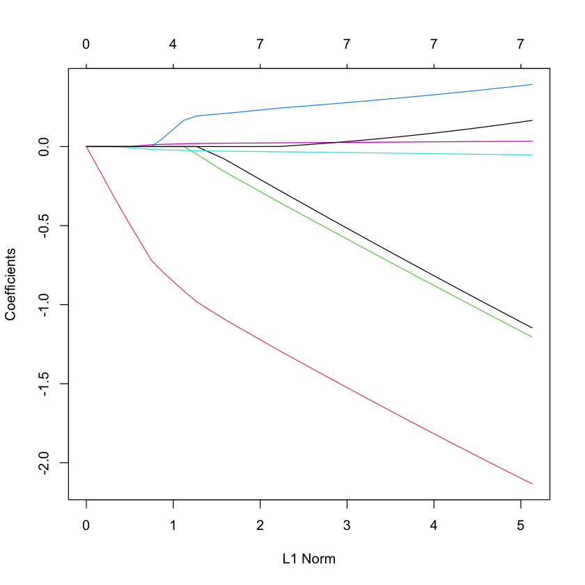
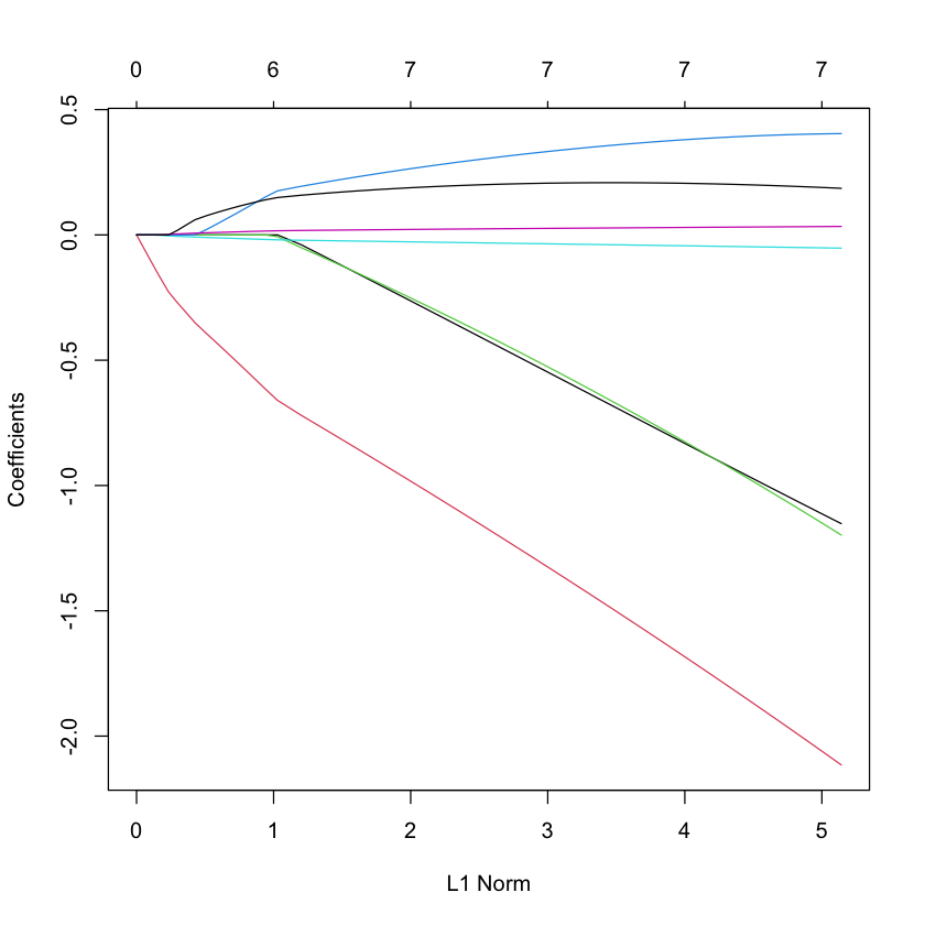
LASSO
library(glmnet)
M = coxph(Surv(time, status) ~ ., data=brainCancer)
D = model.frame(M) # treats diagnosis as continuous
X = model.matrix(M)[,-1]
Y = D[,1]
plot(glmnet(X, Y, family='cox'))
Loading required package: Matrix
Loaded glmnet 4.0-2
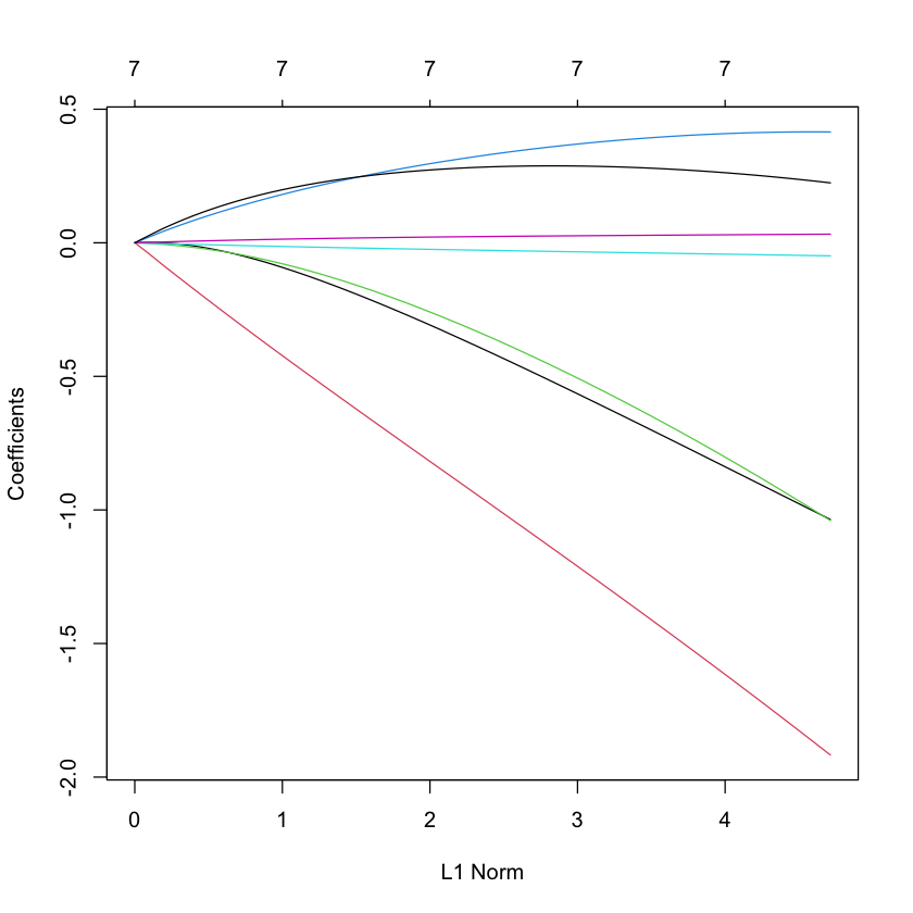
Ridge
plot(glmnet(X, Y, family='cox', alpha=0))
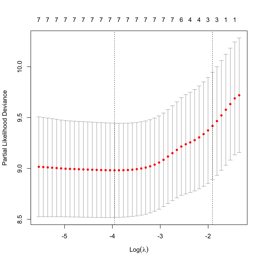
Cross-validation score
For logistic regression we looked at cross-validated Binomial deviance.
Misclassification error is a good metric when we don’t believe our logistic regression model.
For Cox model, we have a negative (partial) log-likelihood (which we can take to be \(DEV/2\)). What is analog of misclassification error for Cox?
Harrell’s concordance score (no ties)
A Cox model produces scores \(\widehat{\eta}=X\widehat{\beta}\).
Cox model indicates that higher \(\eta\) should yield sooner failure time.
For scores \(\eta\) and times \(T\), a pair is concordant if \(\eta_i < \eta_j\) and \(T_i > T_j\). But we have censored data…
We can compare pairs \((i,j)\) that are both uncensored (i.e. \(\delta_i=\delta_j=1\)).
If \(O_i > O_j\) and \(\delta_j=1\) then we know \(T_i > T_j\) and can check concordance
If \(O_i < O_j\) and \(\delta_j=1\) then we don’t know that \(T_i \overset{?}{>} T_j\)…
Leads to $\( \begin{aligned} C(\eta, O, \delta) &= \frac{\sum_{i,j:\delta_j=1} 1_{\{\eta_i < \eta_j\}} 1_{\{O_i > O_j\}} d_j(\delta)}{\sum_{i,j: \delta_j=1} 1_{\{O_i > O_j\}} d_j(\delta)} \\ &= \frac{\sum_{i,j} 1_{\{\eta_i < \eta_j\}} 1_{\{O_i > O_j\}} d_j(\delta)}{\sum_{i,j} 1_{\{O_i > O_j\}} d_j(\delta)} \\ \end{aligned} \)$
plot(cv.glmnet(X, Y, family='cox', type.measure='C'))

Verifying proportional hazard assumption
For a categorical variable, the lines cannot cross and should be some baseline function raised to different powers: in category \(j\) $\( S_j(t) = \exp\left(-c_j H(t)\right) = (\exp(-H(t))^{c_j} \)$
So if \(c_j > c_k\), then \(S_j(t) \leq S_k(t) \forall t\).
Crossing survival curves \(\implies\) proportional hazards cannot hold.
plot(survfit(Surv(time, status) ~ diagnosis, data=brainCancer), lty=c(1:4))

plot(survfit(Surv(time, status) ~ sex, data=brainCancer), lty=c(1:2))

Verifying proportional hazard assumption
Difficult to produce such plots for models like
M2with more than one categorical predictor.Need a way to detect departures from proportional hazards model.
Alternative model, allow \(\beta\) to vary with time: $\( h_{\beta}(t;x) = h_0(t) \exp(X^T\beta(t)) \)$
Proportional hazards for feature \(j\) is equivalent to \(\beta(t) \equiv \beta_j\)
Residuals (continued)
Schoenfeld residuals: for each event \(T_i,\delta_i=1\) $\( S_i(\beta) = X_i - E_{\beta,i}[X] \)$
Total score $\( \sum_{i:\delta_i=1} S_i(\beta). \)$
Scaled Schoenfeld residual $\( S_i^*(\beta) = \text{Var}_{\beta,i}[X]^{-1}S_i \)$
\(S^*_i\) can be related to Taylor series for \(\beta(t)\) in time dependent alternative…
Using Schoenfeld residuals to test PH
Suppose \(\beta=\beta(t)\) and write the log-likelihood as
where
If we were to conduct a “score test” of \(H_0:\beta(t) \equiv \beta\) we would plugin the best fitting constant \(\beta\) (i.e. the Cox MLE).
Our likelihood depends only on \(\{\beta(T_i): \delta_i=1\}\) so consider perturbations $\( \beta(T_i) = \widehat{\beta} + \zeta_i \)$
Further, each \(\delta_i\) only shows up in \(\ell_i(\beta)\) and
Residual plot
A “reasonable guess” at \(\delta_i\) maximizes LHS above
Formally, these are one-step estimators of \(\zeta_i\) from the MLE under \(H_0\)…
Under null, plot of
should look flat if \(\beta_j(t) \equiv \beta_j\).
par(mfrow=c(2,1))
plot(cox.zph(M2))
M2
Call:
coxph(formula = Surv(time, status) ~ sex + diagnosis, data = brainCancer,
    subset = subs)

                       coef exp(coef) se(coef)      z        p
sexMale              0.0353    1.0359   0.3617  0.098   0.9223
diagnosisLG glioma  -1.1108    0.3293   0.5632 -1.972   0.0486
diagnosisMeningioma -1.9822    0.1378   0.4382 -4.524 6.07e-06
diagnosisOther      -1.1891    0.3045   0.5113 -2.325   0.0200

Likelihood ratio test=23.51  on 4 df, p=0.0001003
n= 87, number of events= 35

Formal test of PH assumption
To test \(H_0:\beta_j(t) \equiv \beta_j\) one can test whether the slope is zero in such plots. (Variance of slope estimator?)
Yields one degree of freedom tests.
cox.zph(M2)
          chisq df    p
sex       0.671  1 0.41
diagnosis 1.337  3 0.72
GLOBAL    1.951  4 0.74
cox.zph(M3)
           chisq df    p
sex       0.9708  1 0.32
ki        0.0547  1 0.81
diagnosis 1.1849  3 0.76
gtv       0.1370  1 0.71
GLOBAL    2.5483  6 0.86