Lecture 7: Variability#
STATS 60 / STATS 160 / PSYCH 10
Concepts and Learning Goals:
Variability of distributions
Intuition for variability from histograms
Common measures of variability:
Variance and Standard Deviation
Quantiles
Announcements:
You will have 1 week for quiz regrade requests.
The 4:30-5:20PM discussion section only has 6 students.
Variability#
Last week, you learned about them mean and median.
Both measure where the center of a distribution (the data) is, for different notions of centering.
Many times, we don’t just care where the center of the distribution is; we also want to know about the variability of the data.
Are most of the samples close to the center (mean/median), or not?
What is the “typical range” the data falls into?
Why care about variability?#
Question: think of examples of scenarios where you care not only where the data is centered, but also what the variability is.
Medicine: you know the average life expectancy, given a diagnosis. But what are the best/worst case scenarios?
Exams: you know the class average, and you know your score. But how do you really compare to the rest of the class?
Investments: you are trying to decide if you should invest in a stock. You know the historical average annual rate of return. But is it possible that there will be a big loss?
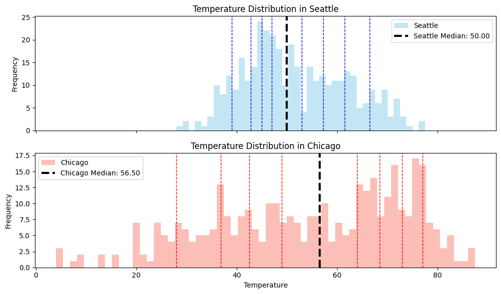
Example 1: daily temperatures in different cities#
Recounting the example from lecture 5, below are the overlayed histograms of daily average temperatures in two cities in 2024-2025.
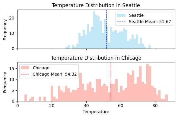
The means of the two cities are very close, but the distributions are very different.
Qualitatively, the temperature in Chicago exhibits greater variability.
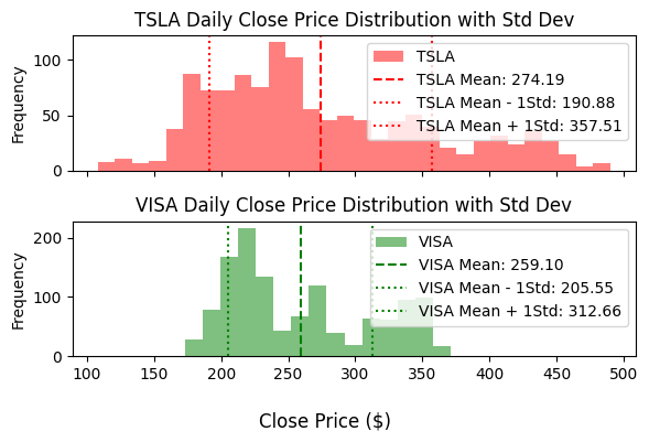
Example 2: stock prices#
These histograms show the daily closing prices of Visa (VISA) and Tesla (TSLA) stock for the last 5 years.
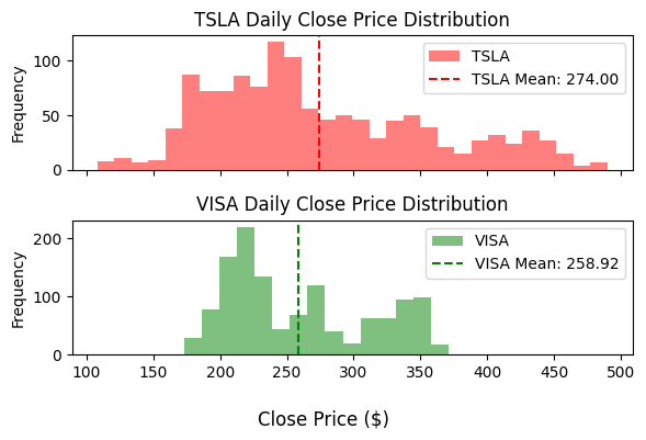
The means are very close, but qualitatively, the TSLA price exhibits greater variability.
How should we measure variability?#
We saw two examples of distributions with similar means, but different levels of variability.
Question: how could we measure variability? Suggest a quantitative measure.
Variance#
A common quantitative summary of variability is the variance.
If our datapoints are \(x_1,\ldots,x_n\), and their mean is \(\bar{x} = \frac{x_1+x_2 + \cdots + x_n}{n}\),
the variance is the average squared distance to the mean:
Practice with the variance#
The variance is the average squared distance to the mean:
Question: Calculate the variance of the rowers’ heights. What are the units?
\(\bar{x}= 70.55\mathrm{in}\) ; \(\bar{\sigma}^2 = 14.47 \mathrm{in}^2\).
Standard Deviation#
The standard deviation is the square root of the variance:
If the data has the units \(u\), then the variance has the units \(u^2\).
The units of the variance are incompatible with the units of the data.
For this reason, if you want a measure of variability that you can compare to the mean, you should use the standard deviation rather than the variance.
Question: Calculate the standard deviation of the rowers’ heights.
\(\sigma = 3.80\mathrm{in}\).
Variability and risk#
Suppose someone offers you a choice between:
A gift of $100
The chance to flip a fair coin for $300.
What would you choose, and why?
We can think of the outcomes in each scenario as datapoints in two different distribution:
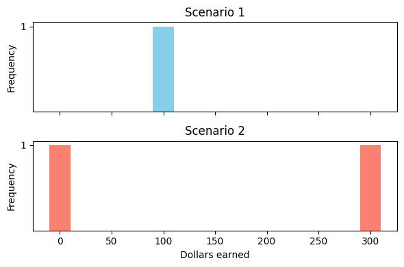
Scenario 1 is a distribution containing exactly one datapoint: $100.
Scenario 2 is a distribution with two datapoints: $0 (tails), $300 (heads)
Question: calculate the mean and standard deviation of your earnings in each scenario.
Scenario |
Mean |
Standard Deviation |
|---|---|---|
1 |
$100 |
$ 0 |
2 |
$150 |
$ 150 |
Example 1: daily temperature#
Mean and Standard Deviation in temperature in 2024-2025:
City |
Mean Temperature |
Standard Deviation |
|---|---|---|
Seattle |
\(51.7^{\circ} F\) |
\(10.3^{\circ} F\) |
Chicago |
\(54.3^{\circ} F\) |
\(19.0^{\circ} F\) |
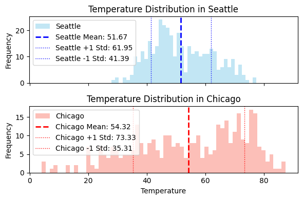
The standard deviation of temperature in Chicago is about twice as much as that of Seattle.
Example 2: stock prices#
Mean and Standard Deviation in closing value for the last 5 years:
Stock |
Mean Value |
Standard Deviation |
|---|---|---|
TSLA |
$274.60 |
$83.24 |
V |
$258.92 |
$53.54 |
The standard deviation of Tesla stock is about 30% of its mean value.
The standard deviation of Visa stock is about 20% of its mean value.
Aside: the ratio of the standard deviation to the mean only makes sense as a measurement of variability for non-negative data.
Standard deviation & outliers#
Sometimes, the standard deviation can be large because of one outlier.
Example: The following dataset gives section attendance for each of the 5 sections of STATS60 this week:
TA |
Attendance |
|---|---|
Cole |
20 |
Junyi |
6 |
Leda |
27 |
Skyler |
25 |
Valerie |
21 |
The mean is 19.8, the standard deviation is 7.3.
If we remove the outlier of Junyi’s section:
the mean is 23.3, the standard deviation is only 2.9.
Discussion#
Question: Do you think the standard deviation is a satisfying measure of variability? What is it conveying? What is it not conveying?
The standard deviation can be large because of the influence of outliers. It can be a “pessimistic” notion of variability.
A guarantee for the standard deviation#
Most samples are within a few standard deviations of the mean!
The following fact is called Chebyshev’s inequality:
For any \(t > 0\), at most a \(1/t^2\) fraction of datapoints are more than \(t\) standard deviations away from the mean.
For example, this implies that 75% of the datapoints are no more than \(2\) standard deviations away from the mean (Chebyshev’s inequality with the choice \(t = 2\)).
You’d see how to prove and use this fact in an intro probability course, like STATS 117/118.
Quantiles#
Quantiles tell us the fraction of the data that falls in each range. They give us a more complete picture of variability.
The \(k\)-quantiles of a distribution are the \(k-1\) numbers which partition the histogram into \(k\) equal-sized parts:
Depicted here are the \(10\)-quantiles, also known as deciles.
Other commonly used quantiles are the quartiles (\(4\)-quantiles), and percentiles (\(100\)-quantiles).
Using quantiles to measure variability#
Question: How can we use quantiles to measure variability?
We can measure distance between quantiles (the “width” of quantiles), or between quantiles and the mean.
For example, the distance from the \(10\)th percentile to \(90\)th percentile:
City |
Mean Temp |
Std. Dev |
10th Percentile |
90th percentile |
10-90 percentile window |
|---|---|---|---|---|---|
Seattle |
\(51.7^{\circ F}\) |
\(10.3^{\circ F}\) |
\(39^{\circ F}\) |
\(66.5^{\circ F}\) |
\(27.5^{\circ F}\) |
Chicago |
\(54.3^{\circ F}\) |
\(19.0^{\circ F}\) |
\(28.0^{\circ F}\) |
\(77.0^{\circ F}\) |
\(49^{\circ F}\) |
Another way to think about quantiles#
Question: How does the information we get from the standard deviation differ from the information we get from the quantiles?
The quantiles give us a better sense of the shape of the distribution.
They also exactly tell us what percent of datapoints fall in a range.
For example: 80% of data points in the histogram fall between the 10th and 90th percentile.
Question: Why?
City |
10th |
90th |
Window Size |
|---|---|---|---|
Seattle |
\(39^{\circ F}\) |
\(66.5^{\circ F}\) |
\(27.5^{\circ F}\) |
Chicago |
\(28.0^{\circ F}\) |
\(77.0^{\circ F}\) |
\(49^{\circ F}\) |
In each city, you can reasonably expect that 80% of the time, the temperature will be in the 10-90th percentile window.
This also gives us a sense of the variability.
Recap#
Concept of variability
Common measures of variability:
Variance and Standard Deviation
Quantiles