Lecture 22: Estimation#
Concepts and Learning Goals:
Estimating an unknown quantity by sampling
Standard deviation of an estimate
Confidence intervals
Recap#
Hypothesis testing#
A p-value is the probability of finding a result at least as extreme/surprising, if outcomes happened by random chance alone.
The null hypothesis corresponds to “no effect.”
The alternative hypothesis corresponds to “an effect.”
Small p-value → evidence against the null hypothesis.
Experiments#
The best way to determine causality is to run a randomized experiment.
This is the gold-standard for inferring a causal relationship between a treatment and an outcome.
Hypothesis testing (potential outcomes, permutation tests) can be used to analyze a randomized experiment.
In observational studies the treatment and control groups might not be comparable and this leads to confounding.
Estimation#
Kissing right#
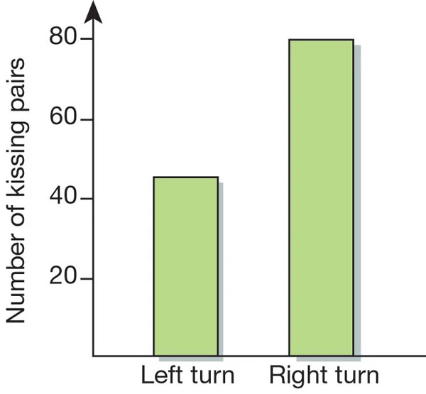
A Nature Communication piece investigates whether couples have a tendency to turn their heads left or right when kissing.
The researchers observed couples in public places and recorded which way they turned their heads when kissing.

Study results#
What is the parameter of interest for this study?
Answer: the parameter of interest is the long run proportion of couples who would turn their heads right when kissing.
Out of 124 couples, 80 turned their heads to the right.
Hypothesis test#
Using the material from week 6, we can test the hypothesis \(H_0 : \pi = 0.5\).
We can use the one-proportion applet.
The p-value is very small. What can we conclude about the null hypothesis?
Another hypothesis test#
By most estimates about 90% of people are right-handed.
Maybe people tend to turn towards their dominant hand.
How could this be formulated as a hypothesis?
Answer: The null hypothesis would be \(H_0 : \pi = 0.9\).
Lets’s use the one-proportion applet again.
The p-value is again very small.
A question#
We have strong evidence against both \(\pi = 0.5\) and \(\pi = 0.9\).
But what would be a plausible value of \(\pi\) based on the data?
Answer: \(\frac{80}{124} \approx 0.66\) which is the proportion of couples who kissed right in the sample.
The sample proportion is called an estimate of \(\pi\).
Estimation#
Populations and parameters#
In general, suppose we want to ask a large group of people a yes/no question.
Example: ask Stanford undergraduate students if they support the proctoring pilot.
This defines a population (current Stanford undergraduates) and a parameter \(\pi\) (the proportion of undergraduates who support the proctoring pilot).
Sampling#
If we asked every person in the population, then we would know \(\pi\).
But this would be time-consuming and expensive (imagine asking every Stanford undergraduate).
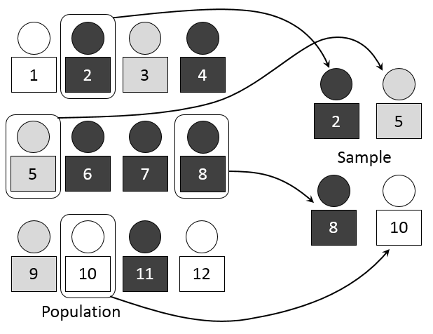
Instead, we could take a sample from the population.
Estimating from a sample#
Suppose we select \(n\) people from the population uniformly at random (\(n\) random Stanford students).
Then we ask them the yes/no question (do you support the proctoring pilot).
If \(m\) out of \(n\) answer yes, then our estimate of \(\pi\) is
\[\hat{\pi}_n = \frac{m}{n}\]The “hat” on \(\hat{\pi}_n\) is to emphasize that it is an estimate. The \(n\) in \(\hat{\pi}_n\) is the sample size.
How good is the estimate?#
True or false: \(\hat{\pi}_n = \pi\)?
Answer: false, most of the time we will have \(\hat{\pi}_n \neq \pi\).
The estimate \(\hat{\pi}_n\) is random: if we had sampled different students, then we would get a different value of \(\hat{\pi}_n\).
We want to know how close \(\hat{\pi}_n\) is to \(\pi\).
Distribution of \(\hat{\pi}_n\)#
The distribution of \(\hat{\pi}_n\) depends on two things: the sample size \(n\) and the parameter \(\pi\).
How do you expect the distribution of \(\hat{\pi}_n\) to change if the sample size \(n\) increased?
Answer: The variability in the distribution should decrease: \(\hat{\pi}_n\) should get closer to \(\pi\).
How would the distribution of \(\hat{\pi}_n\) change if \(\pi\) increased?
Answer: the distribution would shift to the right to stay centered at \(\pi\).
Simulation for \(\hat{\pi}_n\)#
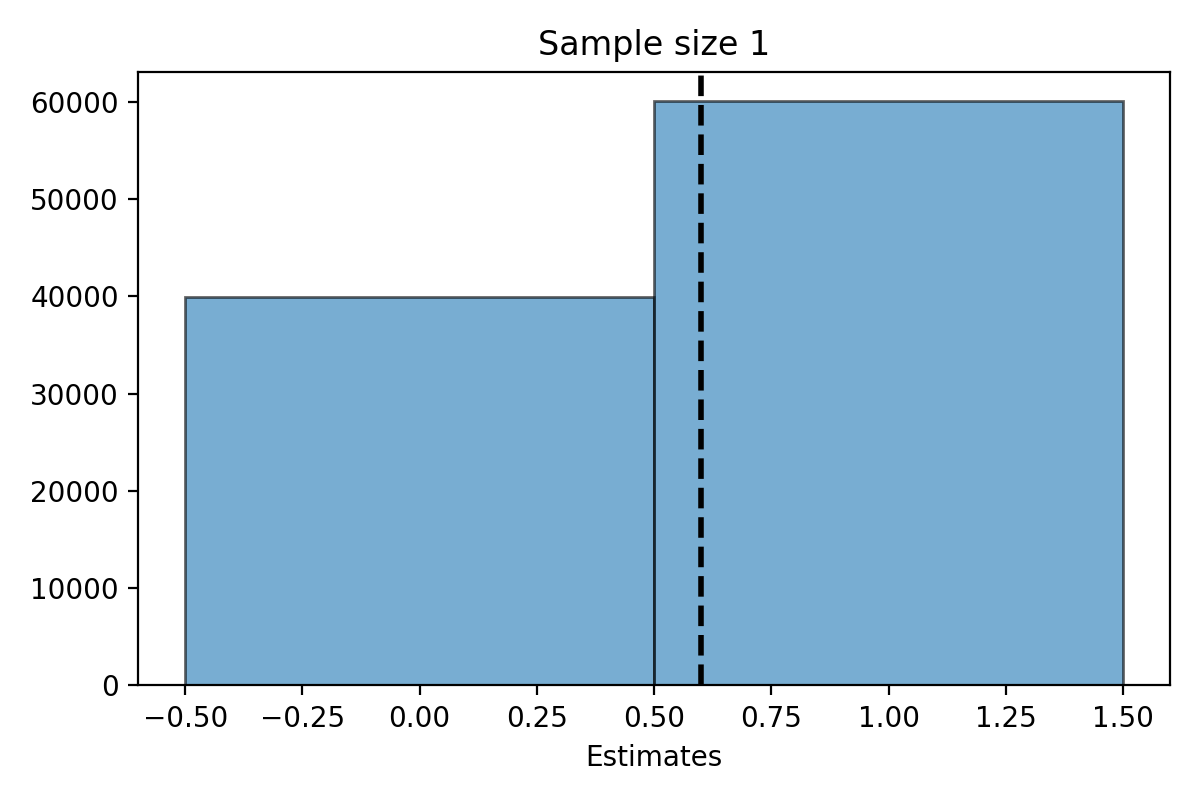
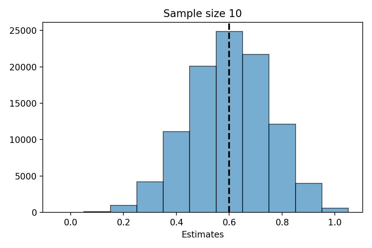
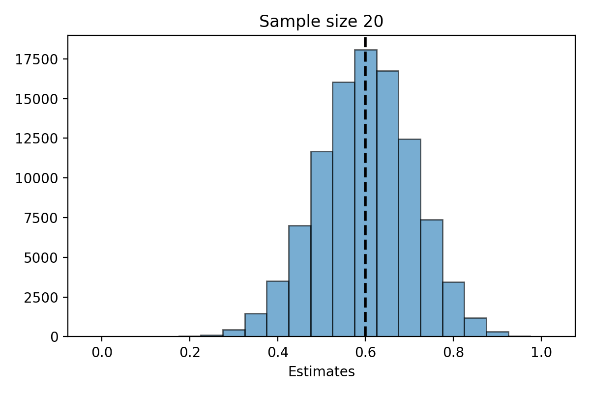
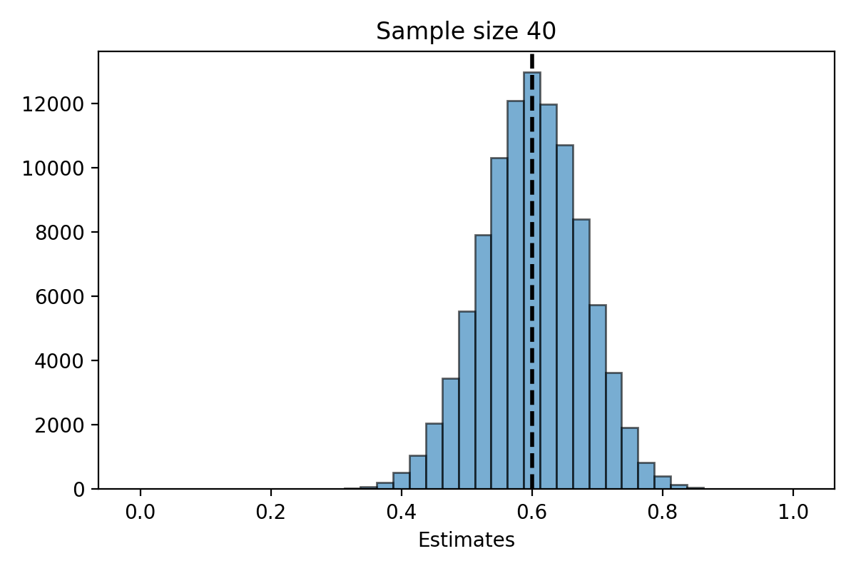
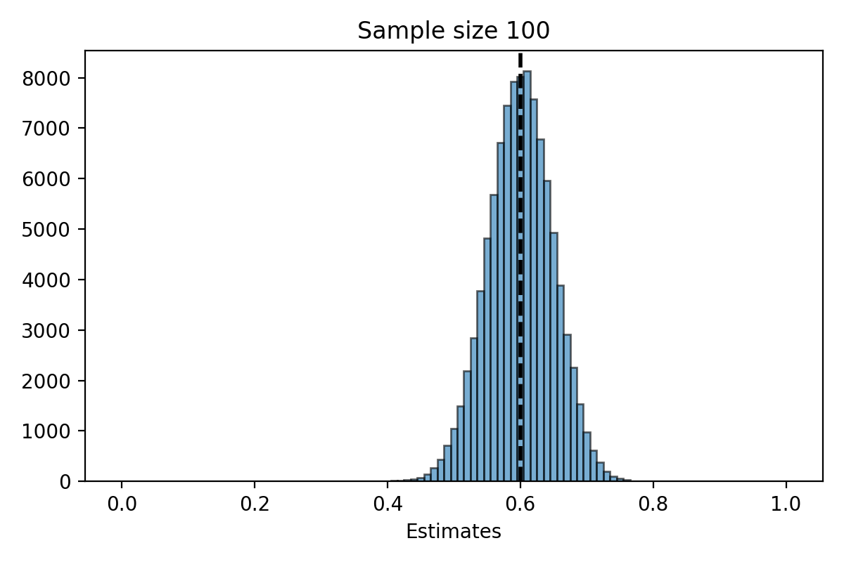
Suppose that we know \(\pi=0.6\) (60% of Stanford student support the proctoring pilot).
We can then do a simulation to look at the distribution of \(\hat{\pi}_n\) for different values of \(n\).
Simulation for \(n=1\)#
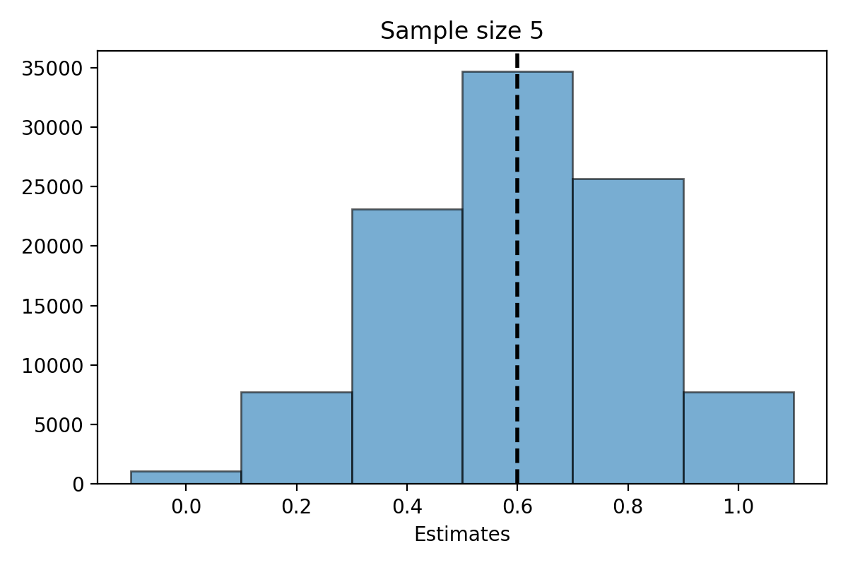
Simulation for \(n=5\)#
Simulation for \(n=10\)#
Simulation for \(n=20\)#
Simulation for \(n=40\)#
Simulation for \(n=100\)#
Simulation summary#
What do you notice about the distribution of \(\hat{\pi}_n\)?
The distribution of the estimate \(\hat{\pi}_n\) is centered at the parameter \(\pi\).
The expected value of \(\hat{\pi}_n\) is \(\pi\).
The distribution of \(\hat{\pi}_n\) is less spread out as \(n\) gets bigger.
The variability of \(\hat{\pi}_n\) decreases as \(n\) gets bigger.
When \(n\) is large, the distribution of \(\hat{\pi}_n\) looks “bell shaped.”
Standard deviation#
Standard deviation recap#
In lecture 7, you saw that the standard deviation was one way to measure the variability of a distribution.
How does the standard deviation of \(\hat{\pi}_n\) change as \(n\) increases?
Answer: the standard deviation decreases as the sample size increases. The distribution becomes less variable/spread-out.
Sample size matters: larger sample size means lower standard deviation.
Standard deviation of \(\hat{\pi}_n\)#
There is an exact formula for the standard deviation of \(\hat{\pi}_n\).
\[\text{Standard deviation of }\hat{\pi}_n = \sqrt{\frac{\pi(1-\pi)}{n}} \]\(\sqrt{\pi(1-\pi)}\) is the standard deviation of \(\hat{\pi}_1\) (just asking one person).
In a sample of size \(n\), the standard deviation is a factor of \(\frac{1}{\sqrt{n}}\) times smaller than just asking one person.
Computing the standard deviation#
The parameter \(\pi\) appears in the formula for the standard deviation (\(\sqrt{\frac{\pi(1-\pi)}{n}}\)). But we don’t know \(\pi\)!
We can use the estimate \(\hat{\pi}_n\): $\(\text{Standard deviation of }\hat{\pi}_n \approx \sqrt{\frac{\hat{\pi}_n(1-\hat{\pi}_n)}{n}} \)$
Kissing right#
In the kissing right study, \(n = 124\) and \(\hat{\pi}_n = 0.66\)
Let’s use \(\hat{\pi}_n\) to compute the standard deviation:
\[\sqrt{\frac{\hat{\pi}_n(1-\hat{\pi}_n)}{n}} = \sqrt{\frac{0.66 \times 0.34}{124}} = 0.042\]Interpretation: the average distance between \(\hat{\pi}_n\) and the parameter \(\pi\) is around \(0.042\)
The normal approximation#
Bell shaped distribution#
For large samples, the distribution of \(\hat{\pi}_n\) is “bell shaped”.
This bell shape is described by the “normal distribution.”
The normal distribution#
When \(n\) is large enough, the distribution of \(\hat{\pi}_n\) is close to the normal distribution.
The normal distribution lets us use the 68-95-99 rule for \(\hat{\pi}_n\).
This helps us be more precise when we talk about how close \(\hat{\pi}_n\) is \(\pi\).
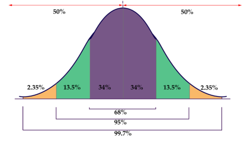
68-95-99 rule#
The 68-95-99 rule states that:
With 68% probability: \(\hat{\pi}_n\) is within one standard deviation of \(\pi\).
With 95% probability: \(\hat{\pi}_n\) is within two standard deviations of \(\pi\).
With 99% probability: \(\hat{\pi}_n\) is within three standard deviations of \(\pi\).
Remember: the standard deviation of \(\hat{\pi}_n\) is \(\sqrt{\frac{\pi(1-\pi)}{n}}\)
68-95-99 rule visualized#
68-95-99 rule: example#
Suppose \(\pi=0.6\) and \(n=100\)
The standard error of \(\hat{\pi}_n\) is
\[\sqrt{\frac{\pi(1-\pi)}{n}} = \sqrt{\frac{0.6 \times 0.4}{100}} = 0.049\]With 95% probability, \(\hat{\pi}_n\) will be within \(2 \times 0.049=0.098\) of \(\pi=0.6\)
With 95% probability \(\hat{\pi}_n\) will be between \(0.6 - 0.098=0.502\) and \(0.6 + 0.098 = 0.698\)
How large does \(n\) need to be?#
A rule of thumb, is that there should be at least 10 “yesses” and 10 “nos” in the sample to apply the normal approximation.
For the kissing right study: there were 80 couples who turned right and 44 couples who turn left. The normal approximation can be used.
In general, the normal approximation gets more accurate for large \(n\) and for proportions closer to \(0.5\).
Confidence intervals#
Kissing right#
In the kissing right study, \(\hat{\pi}_n = 0.66\) and the standard deviation of \(\hat{\pi}_n\) is \(0.042\)
By the 68-95-99 rule: with 95% probability \(\hat{\pi}_n\) is within \(2 \times 0.042\) of \(\pi\)
Based on \(\hat{\pi}_n\), a plausible range for \(\pi\) would be between
\[0.66 - 2\times 0.042= 0.576\]
and $\(0.66+2\times 0.042 = 0.744\)$
Confidence intervals#
A confidence interval is a collection of plausible values of the parameter based on the data.
Example: \([0.576, 0.744]\) is a confidence interval for the proportion of couples who turn right when kissing (\([a,b]\) represents the interval of numbers between \(a\) and \(b\)).
The confidence interval \([0.576, 0.744]\) is called a 95% confidence interval (we used two standard deviations).
We are 95% confident that \(\pi\) is between 0.576 and 0.744.
Confidence intervals questions#
Question: would a 99% confidence interval be bigger or smaller than a 95% confidence interval?
Answer: The 99% confidence interval will be bigger. To have higher confidence, we have to include more values.
Question: how could we compute a 99% confidence interval based on the kissing right data?
Answer: by the 68-95-99 rule, we are 99% confident that \(\pi\) is between $\(0.66 - 3\times 0.042= 0.534\)\( and \)\(0.66+3\times 0.042 = 0.786\)$
Confidence intervals and hypothesis tests#
The confidence interval \([0.576, 0.744]\) contains the values of \(\pi\) which we would not reject in a hypothesis test with threshold 0.05
Example 1: we rejected \(H_0: \pi=0.5\) and \(0.5\) is not in \([0.576, 0.744]\)
Example 2: we would not reject \(H_0 : \pi=0.6\) because \(0.6\) is in \([0.576, 0.744]\) (one-proportion applet)
Practice#
A student wants to assess if her dog Muffin is more likely to chase a red ball or a blue ball when both are rolled.
The student rolls both balls 96 times and Muffin chased the blue ball 52 times.
What is the parameter of interest?
The parameter \(\pi\) is the long-run probability of Muffin chasing the blue ball.
Practice continued#
What is the estimate of \(\pi\)?
The estimate of \(\pi\) is the sample proportion \(\hat{\pi}_n = \frac{52}{96} = 0.54\).
What is the standard deviation of \(\hat{\pi}_n\)?
The standard deviation of \(\hat{\pi}_n\) is \(\sqrt{\frac{\hat{\pi}_n(1-\hat{\pi}_n)}{n}} = 0.056\)
How would you compute a 95% confidence interval for \(\pi\)?
By the 68-95-99 rule: $\([0.54 - 2\times 0.056, 0.54 + 2 \times 0.056] = [0.428, 0.652]\)$
Confidence intervals and sample size#
To use the 68-95-99 rule to make confidence intervals, the sample size needs to be large.
Roughly: there should be at least 10 “yesses” and “nos”.
In math: you need \(n \hat{\pi}_n \ge 10\) and \(n(1-\hat{\pi}_n) \ge 10\).
For smaller sample sizes, the normal approximation is not very accurate, but there are other methods that can be used to make confidence intervals.
Summary#
Sampling and estimation#
Samples can be used to estimate parameters.
Population ↔ parameter ↔ \(\pi\)
Sample ↔ estimate ↔ \(\hat{\pi}_n\)
The distribution of \(\hat{\pi}_n\) is centered at \(\pi\) and has standard deviation
\[ \sqrt{\frac{\pi(1-\pi)}{n}} \approx \sqrt{\frac{\hat{\pi}_n(1-\hat{\pi}_n)}{n}} \]Larger sample size ↔ smaller standard deviation ↔ \(\hat{\pi}_n\) is closer to \(\pi\)
Confidence intervals and the normal approximation#
A confidence interval is a collection of plausible values for the parameter.
A confidence interval has a confidence level (for example 95%).
We are 95% confident that a 95% confidence interval contains the parameter.
Confidence intervals can be calculated using the 68-95-99 rule and the normal approximation.