Lecture 23: Estimation for quantitative variables#
Announcements:
Practice quizzes are online.
Please bring a laptop to section tomorrow.
Recap#
Sampling#
Samples can be used to estimate parameters.
Example: sample \(n\) Stanford students and ask if they support the proctoring pilot.
This defines an unknown parameter \(\pi\) (the proportion of all Stanford students who support the proctoring pilot).
And an estimate \(\hat{\pi}_n\) (the proportion of students in the sample who support the proctoring pilot).
Distribution of \(\hat{\pi}_n\)#
The distribution of \(\hat{\pi}_n\) is centered at \(\pi\) and has standard deviation:
\[ \sqrt{\frac{\pi(1-\pi)}{n}} \approx \sqrt{\frac{\hat{\pi}_n(1-\hat{\pi}_n)}{n}} \]Larger sample size ↔ smaller standard deviation ↔ \(\hat{\pi}_n\) is closer to \(\pi\)
Confidence intervals#
A confidence interval is a collection of plausible values for the parameter.
A confidence interval has a confidence level (for example 95%).
We are 95% confident that a 95% confidence interval contains the parameter.
Confidence intervals can be calculated using the 68-95-99 rule and the normal approximation.
Example: proctoring pilot#
Suppose you surveyed \(n=100\) Stanford students and \(55\) of them say they support the proctoring pilot.
What is the estimate \(\hat{\pi}_n\)?
Answer: \(\hat{\pi}_n = \frac{55}{100}=0.55\)
What is the standard deviation of \(\hat{\pi}_n\)?
Answer: $\(\sqrt{\hat{\pi}_n(1-\hat{\pi}_n)/n} = \sqrt{0.55 \times 0.45 / 100} = 0.05\)$
What is a 68% confidence interval for \(\pi\)?
Answer: by the 68-95-99 rule:
\[\hat{\pi}_n \pm \sqrt{\frac{\hat{\pi}_n(1-\hat{\pi}_n)}{n}} = 0.55 \pm 0.05 = [0.5, 0.6]\]
The importance of random sampling#
The previous results are only valid if the sample is drawn randomly.
Each student needs to have the same chance of being selected and students should be sampled independently.
If some students are more likely to be chosen, then \(\hat{\pi}_n\) might be biased.
If the students are not sampled independently, then the formula \(\sqrt{\hat{\pi}_n(1-\hat{\pi}_n)/n}\) is not correct.
More on this on Friday.
Estimation for quantitative variables#
Populations and parameters#
Sometimes, we want to know about something other than a yes or no question.
Instead, we might want to measure a quantitative variable.
We could in theory measure the variable for every observational unit in the population of interest.
This would let us calculate the population mean.
The population mean is a parameter and written as \(\mu\) (a Greek m, pronounced “mu”).
Samples and estimation#
As with polling, it is more efficient to take a sample instead of measuring every observational unit in the population.
Suppose that we randomly sample \(n\) observational units, and measure the quantitative variable for all of them.
This gives \(n\) measurements: \(x_1,x_2,\ldots,x_n\).
The sample mean of \(x_1,\ldots,x_n\) is
\[\hat{\mu}_n = \frac{x_1+x_2+\cdots + x_n}{n} \]
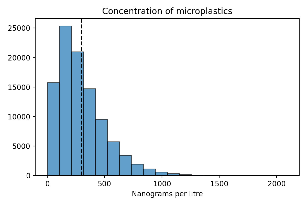
Microplastics#
We want to determine the average concentration of microplastics in Palo Alto tap water.
The concentration is a parameter. It is a fixed unknown quantity \(\mu\).
Estimating \(\mu\) with a sample:
Take \(n\) water samples and measure the microplastics in each. This produces measurements \(x_1,x_2,\ldots,x_n\).
\(x_i\) is the concentration of microplastics in the \(i\) th sample.
Properties of \(\hat{\mu}_n\)#
The estimate is the sample mean: \(\hat{\mu}_n = \frac{x_1+x_2+\cdots + x_n}{n}\)
Like \(\hat{\pi}_n\), the estimate \(\hat{\mu}_n\) is random and most of the time \(\hat{\mu}_n \neq \mu\). But \(\hat{\mu}_n\) should be close to \(\mu\).
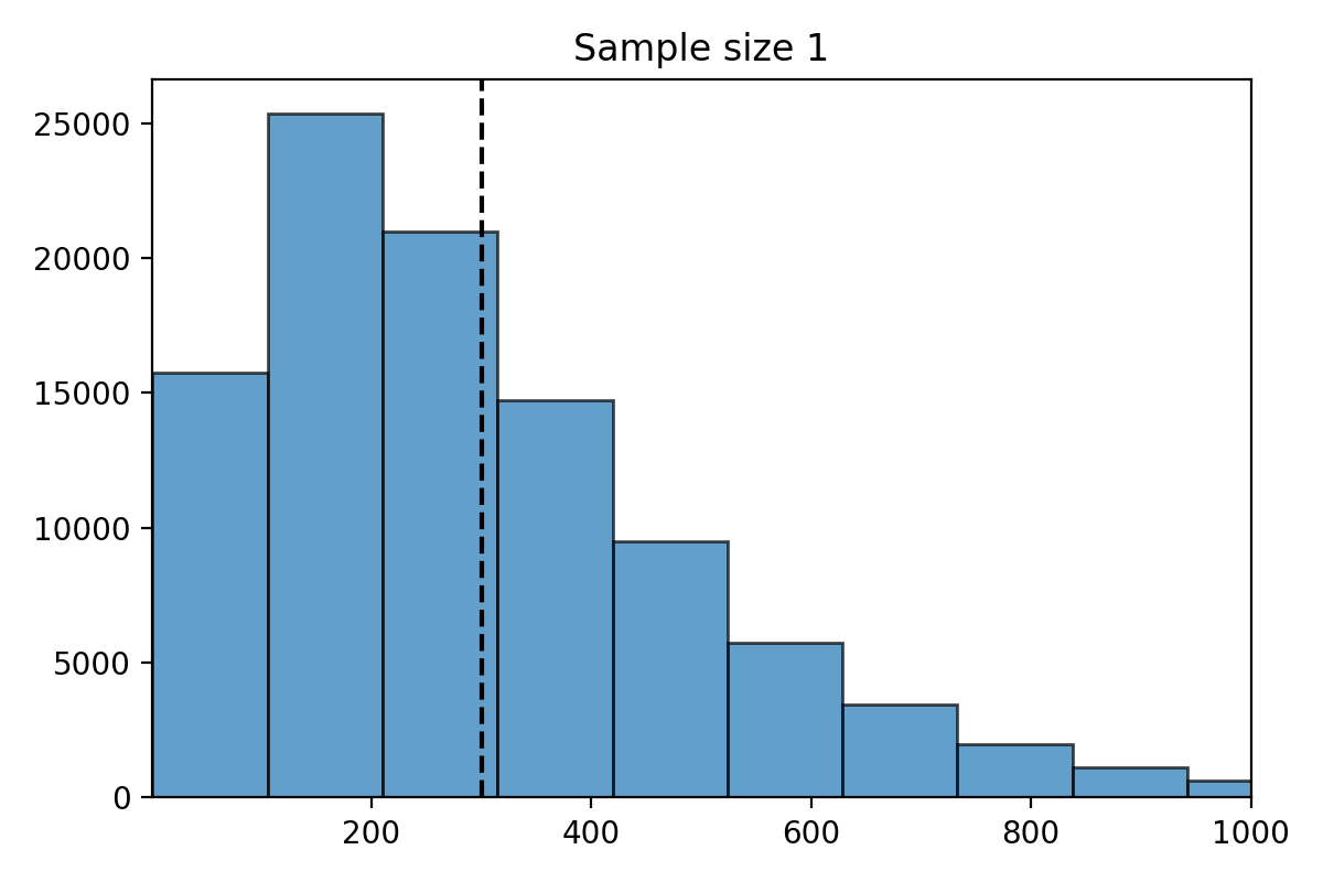
Question: how does the sample size \(n\) effect the distribution of \(\hat{\mu}_n\)?
Answer: if the sample size \(n\) increases, then the variability of \(\hat{\mu}_n\) will decrease. The histogram should become skinnier.
Simulation for \(\hat{\mu}_n\)#
Let’s suppose that we know the distribution of the concentration of microplastics in Palo Alto tap water.
We can do a simulation to see what the distribution of \(\hat{\mu}_n\) looks like for different values of \(n\).
Simulation for \(n=1\)#
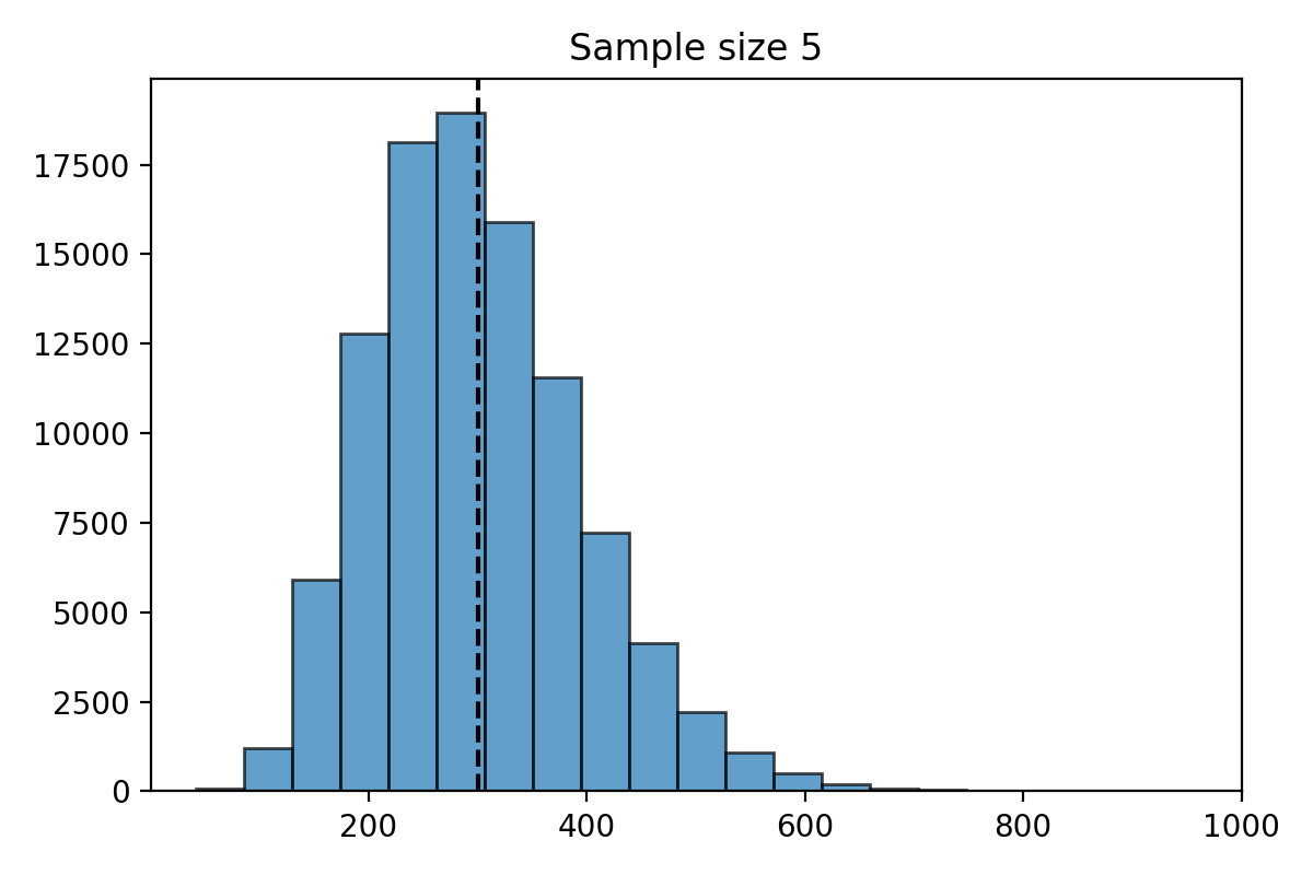
Simulation for \(n=5\)#
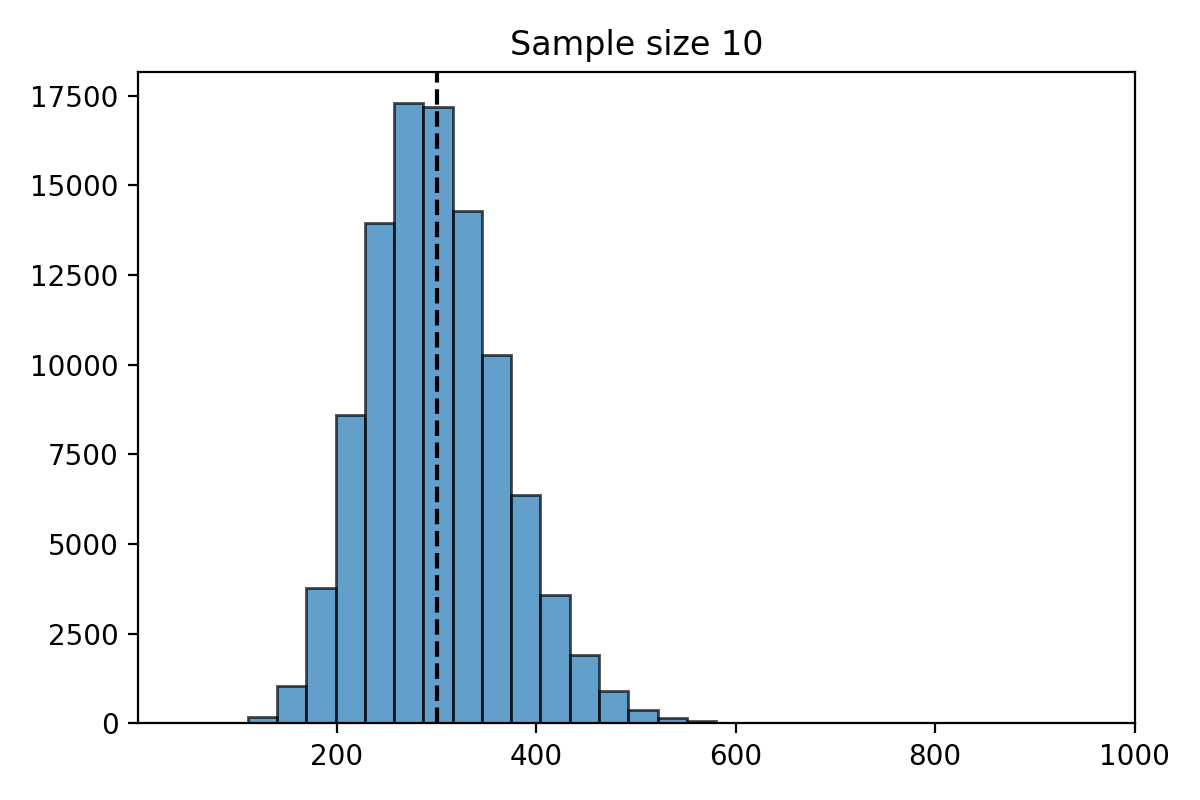
Simulation for \(n=10\)#
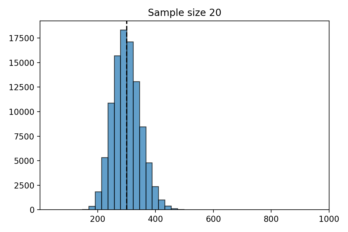
Simulation for \(n=20\)#
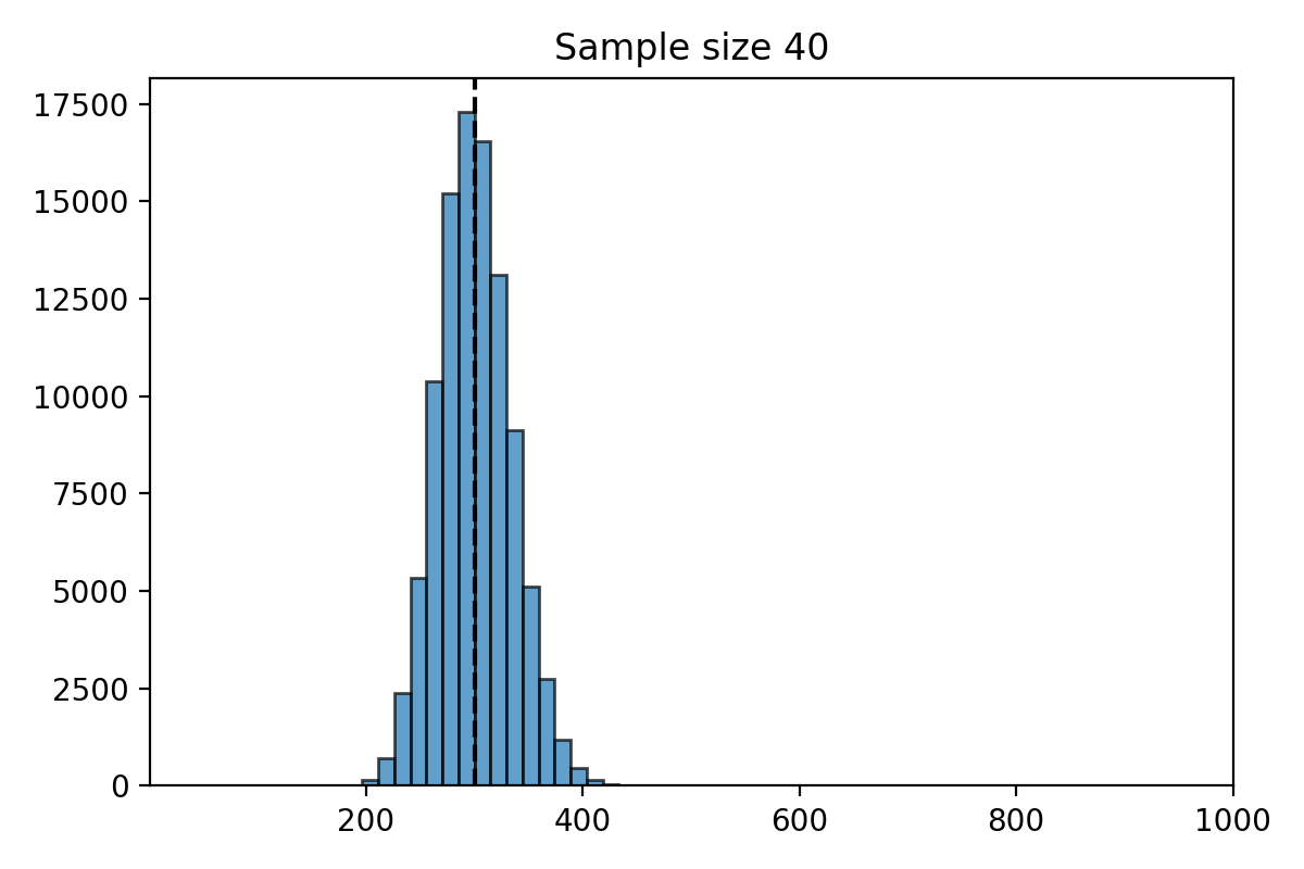
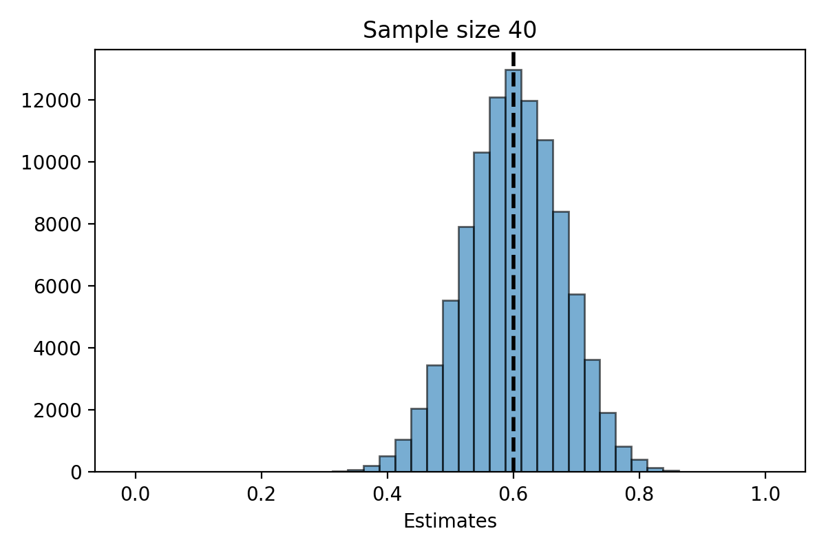
Simulation for \(n=40\)#
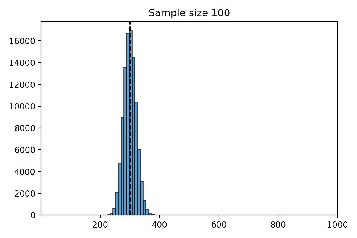
Simulation for \(n=100\)#
Simulation summary#
What do you notice about the distribution of \(\hat{\mu}_n\)?
The distribution of the estimate \(\hat{\mu}_n\) is centered at the parameter \(\mu = 300\).
The expected value of \(\hat{\mu}_n\) is \(\mu\).
The distribution of \(\hat{\mu}_n\) is less spread out as \(n\) gets bigger.
The standard deviation of \(\hat{\mu}_n\) decreases as \(n\) gets larger.
When \(n\) is large, the distribution of \(\hat{\mu}_n\) looks “bell shaped.”
The normal approximation also applies to \(\hat{\mu}_n\)
Comparison to \(\hat{\pi}_n\)#
Distribution of \(\hat{\pi}_n\)
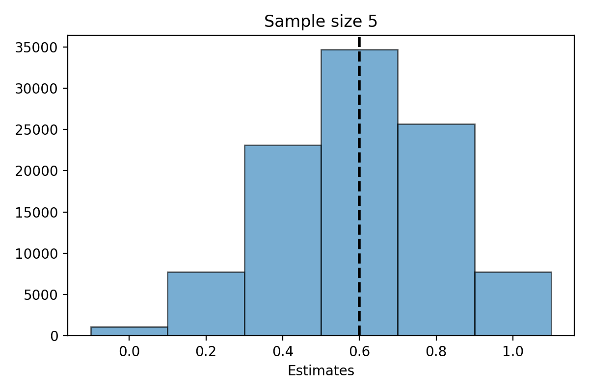
Distribution of \(\hat{\mu}_n\)
Comparison to \(\hat{\pi}_n\)#
Distribution of \(\hat{\pi}_n\)
Distribution of \(\hat{\mu}_n\)
Confidence intervals for \(\mu\)#
Standard deviation of \(\hat{\mu}_n\)#
Let \(\sigma_x\) be the standard deviation of a single sample \(x\).
The standard deviation of the estimate \(\hat{\mu}_n\) is given by:
\[\text{standard deviation of } \hat{\mu}_n = \frac{\sigma_x}{\sqrt{n}}\]As with proportions, the standard deviation of \(\hat{\mu}_n\) is smaller by a factor of \(\frac{1}{\sqrt{n}}\).
Computing the standard deviation#
The standard deviation of a single sample \(\sigma_x\) is not known.
So instead we will estimate it with the sample standard deviation \(\hat{\sigma}_x\).
\[\text{standard deviation of } \hat{\mu}_n \approx \frac{\hat{\sigma}_x}{\sqrt{n}}\]The sample standard deviation \(\hat{\sigma}_x\) can be computed from the sample \(x_1,\ldots,x_n\).
Microplastics#
Suppose that collected \(n=100\) water samples and measured the concentration of microplastics in all of them.
Suppose that the estimate \(\hat{\mu}_n\) is 310 nano grams per litre and \(\hat{\sigma}_x\) is 200 nano grams per litre.
What is the standard deviation of \(\hat{\mu}_n\)?
Answer:
\[\frac{\hat{\sigma}_x}{\sqrt{n}} = \frac{200}{\sqrt{100}} = \frac{200}{10} = 20\]
Normal approximation#
When \(n\) is large, the distribution of \(\hat{\mu}_n\) is close to the normal distribution.
The distribution of the measurements \(x_1,x_2,\ldots,x_n\) might not be close to the normal distribution.
But, the distribution of \(\hat{\mu}_n\) will be close to the normal distribution if \(n\) is big.
68-95-99 rule#
This means we can use the 68-95-99 rule:
With 68% probability: \(\hat{\mu}_n\) is within one standard deviation of \(\mu\).
With 95% probability: \(\hat{\mu}_n\) is within two standard deviations of \(\mu\).
With 99% probability: \(\hat{\mu}_n\) is within three standard deviations of \(\mu\).
Confidence intervals#
We can make confidence interval using the 68-95-99 rule.
In the microplastics example, suppose that \(\hat{\mu}_n=310\) and the standard deviation of \(\hat{\mu}_n\) is \(20\). What is a 95% confidence interval for \(\mu\)?
We are 95% confident that the concentration of microplastics in Palo Alto tap water is between 270 and 350 nanograms per litre.
Mini crosswords#
New York Times Mini crosswords#
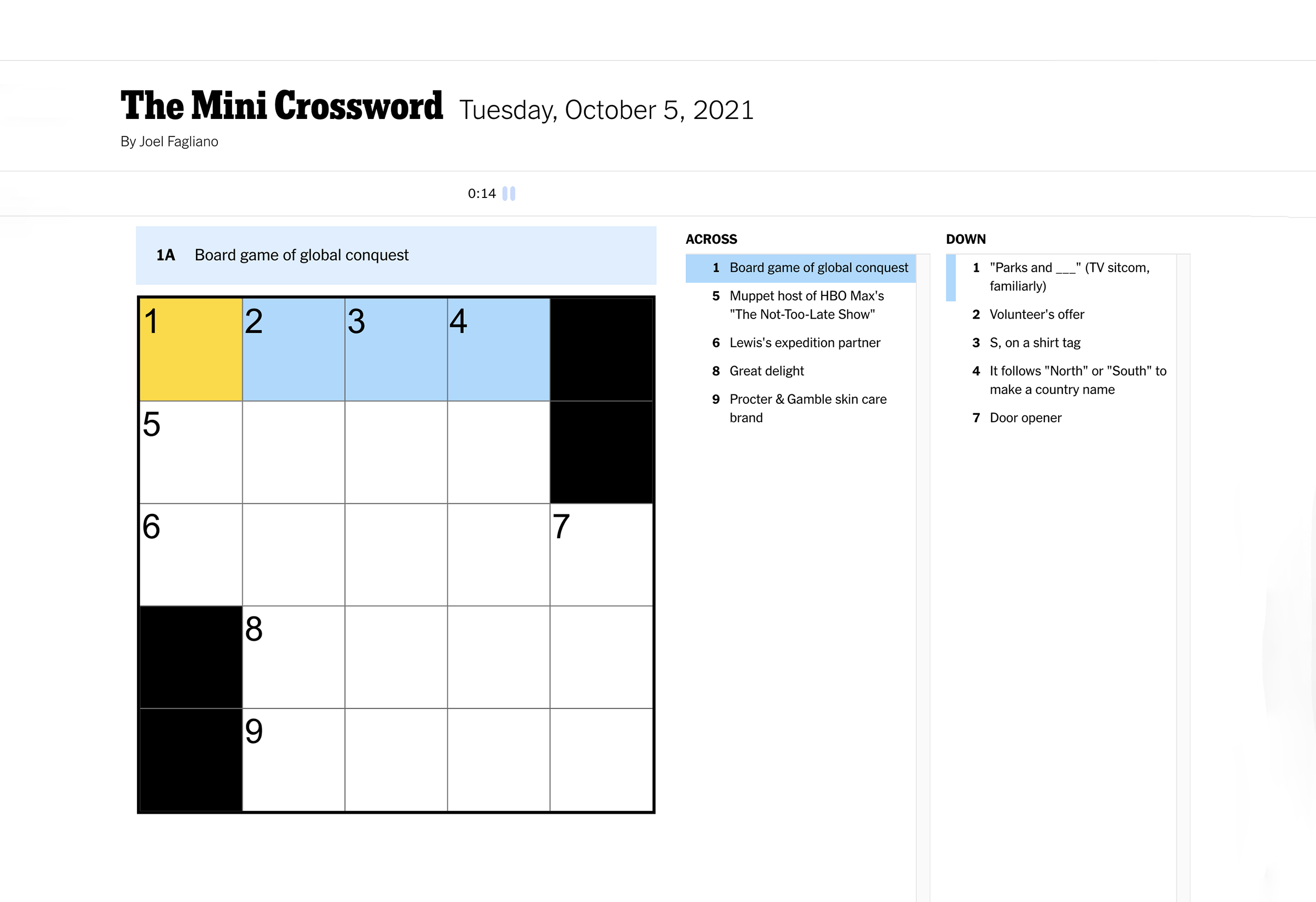
Clikey and Andel#

Data#
Here is a dataset of the time it took us to do the mini crosswords:
date |
Clikey time |
Andel time |
Difference |
Winner |
|---|---|---|---|---|
9-Jul |
42 |
44 |
-2 |
Clikey |
11-Jul |
78 |
55 |
23 |
Andel |
12-Jul |
92 |
107 |
-15 |
Clikey |
13-Jul |
67 |
90 |
-23 |
Clikey |
And so on for a total of \(n=33\) rows.
Estimation#
Let \(x_1,x_2,\ldots,x_n\) be the difference between Clikey and Andel’s crossword times.
We will pretend that \(x_1,x_2,\ldots,x_n\) are a representative sample of the two team’s crossword performance.
Let \(\mu\) be the long-run average difference in crossword times.
The sample mean is \(\hat{\mu}_n\) is \(-7.3\) seconds. Is this evidence that Clikey are better than Andel?
Confidence interval#
The sample mean is \(\hat{\mu}_n=-7.3\) seconds, the sample size is \(n=33\) and the standard deviation of \(x_1,\ldots,x_n\) is \(\hat{\sigma}_x= 75\) seconds. What is a 95% confidence interval for \(\mu\)?
Answer: first calculate the standard deviation of \(\hat{\mu}_n\) which is \(\frac{\hat{\sigma}_x}{\sqrt{n}} = \frac{75}{\sqrt{33}}=13\)
Then use the 68-95-99 rule:
\[\hat{\mu}_n \pm 2\times\frac{\hat{\sigma}_x}{\sqrt{n}} = -7.3 \pm 2 \times 13 = [-33.3, 19.3]\]Based on the confidence interval both \(\mu <0\) (Clikey are better) and \(\mu >0\) (Andel are better) are plausible.
Standard deviation of \(\hat{\mu}_n\)#
Standard deviation and standard error#
Recall that if \(\hat{\sigma}_x\) is the standard deviation of \(x_1,x_2,\ldots,x_n\), then the standard deviation of \(\hat{\mu}_n\) is \(\frac{\hat{\sigma}_x}{\sqrt{n}}\)
It is easy to confuse \(\hat{\sigma}_x\) and \(\frac{\hat{\sigma}_x}{\sqrt{n}}\).
\(\hat{\sigma}_x\) is the standard deviation of just a single measurement (\(n=1\)).
\(\hat{\sigma}_x/\sqrt{n}\) is the standard deviation of the sample mean with a sample size of size \(n\).
\(\hat{\sigma}_x/\sqrt{n}\) is sometimes called the standard error.
Standard deviation and sample size#
The standard deviation of \(\hat{\mu}_n\) is \(\frac{\hat{\sigma}_x}{\sqrt{n}}\).
The standard deviation of \(\hat{\mu}_n\) is proportional to \(\frac{1}{\sqrt{n}}\).
If you double the sample size, then the standard deviation of \(\hat{\mu}_n\) will decrease by a factor of \(\sqrt{2}=1.41\) not by a factor of \(2\).
If you want the standard deviation of \(\hat{\mu}_n\) to decrease by a factor of \(2\), then you need to increase the sample size by a factor of \(2^2=4\).
Computing a required sample size#
The formula \(\frac{\hat{\sigma}_x}{\sqrt{n}}\) can be used to compute the required sample size for a desired level of precision.
In the minis, suppose that Clikey are actually 5 seconds faster on average (\(\mu = -5\)).
How large does \(n\) need to be so that a 95% confidence interval centered at \(-5\) will only include negative numbers? (Assume that \(\hat{\sigma}_x = 75\))
Computing a required sample size#
We need to solve for \(n\) in the equation
\[2 \frac{\hat{\sigma}_x}{\sqrt{n}} = 5 \]Rearranging and using \(\hat{\sigma}_x=75\):
\[\sqrt{n} = \frac{2\hat{\sigma}_x}{5} = 30\]And so \(n = 30^2 = 900\) which is about 2 and a half years of mini crosswords.
Connection to proportions#
Similarities between \(\hat{\pi}_n\) and \(\hat{\mu}_n\)#
The estimates \(\hat{\pi}_n\) and \(\hat{\mu}_n\) have a lot in common:
Both are centered at the population parameters \(\pi\) and \(\mu\).
The standard deviations of \(\hat{\pi}_n\) and \(\hat{\mu}_n\) both decrease with \(n\).
When \(n\) is large, the distribution of \(\hat{\pi}_n\) and \(\hat{\mu}_n\) is close to the normal distribution.
These similarities are not just a coincidence.
Proportions are means#
The sample proportion \(\hat{\pi}_n\) is a special case of the sample mean \(\hat{\mu}_n\).
Let \(x_1,\ldots,x_n\) be measurements where \(x_i=1\) if the \(i\) th person in the sample answered yes and \(x_i=0\) if they answered no.
Then
\[\hat{\mu}_n = \frac{x_1+x_2+\cdots+x_n}{n}=\frac{m}{n} = \hat{\pi}_n \]where \(m\) is the number of people in the sample who answered yes.
Proportions and means#
Most of the results from Monday about \(\hat{\pi}_n\) are a special case of the results for \(\hat{\mu}_n\).
There are two things that are special about \(\hat{\pi}_n\):
The formula \(\sqrt{\frac{\hat{\pi}_n(1-\hat{\pi}_n)}{n}}\) for the standard deviation of \(\hat{\pi}_n\) (for \(\hat{\mu}_n\) the formula is \(\frac{\hat{\sigma}_x}{\sqrt{n}}\))
The rule of thumb that the normal approximation is reasonably accurate when \(\hat{\pi}_n n \ge 10\) and \((1-\hat{\pi}_n)n \ge 10\).
How large should \(n\) be?#
There isn’t a similar rule for the normal approximation for quantitative variables.
The accuracy of the normal approximation depends on both the size of \(n\) and how asymmetric the distribution of \(x_1,\ldots,x_n\) is.
If the distribution is very asymmetric, then \(n\) needs to be larger.
If the distribution is not too “wild”, then \(n=30\) should give good results.
Error bars#
Confidence intervals and error bars#
Confidence intervals are often expressed visually with error bars, like in this figure from Do defaults save lives?
Error bar: warning#
There are different conventions about what is displayed in the error bars.
Sometimes it is a 95% confidence interval, other times it is the standard deviation of \(\hat{\mu}_n\) and other times it is the standard deviation of \(x_1,\ldots,x_n\)!
Any figure with error bars should say how they are calculated.
Uncertainty#
Error bars and confidence intervals are meant to represent uncertainty in an estimate.
For example: 42% of people in Opt-in group consented to be donors, but the population proportion could be between 32% and 52%
In many cases, people focus on the estimate and ignore the error bars and uncertainty.
This has led people to develop alternatives.
How would design a visualization that emphasizes uncertainty?
Hypothetical outcomes plot#
One alternative is a moving image that shows different plausible estimates. More information here.
Confidence intervals conclusions#
Population and sample#
There is a variable \(x\) which we want to measure on observation units in a population.
Our goal is to estimate the population mean \(\mu\) which is a parameter.
We take independent \(n\) samples from the population and record the variable on the sample.
This gives measurements \(x_1,\ldots,x_n\).
The sample mean \(\hat{\mu}_n = \frac{x_1+\cdots+x_n}{n}\) is an estimate of \(\mu\).
Confidence intervals#
A confidence interval for \(\mu\) is a collection of plausible values of \(\mu\).
The estimate \(\hat{\mu}_n\) can be used to make confidence intervals of the form
\[ \hat{\mu}_n \pm 2 \frac{\hat{\sigma}_x}{\sqrt{n}}\]where \(n\) is the sample size and \(\hat{\sigma}_x\) is the standard deviation of \(x_1,\ldots,x_n\).
This produces a 95% confidence interval (2 standard deviations).
For 68% use 1 standard deviation and for 99% use 3 standard deviations.
Confidence intervals theory#
The normal approximation means that
\[\mathrm{Pr}\left[\hat{\mu}_n - \frac{2\hat{\sigma}_x}{\sqrt{n}} \le \mu \le \hat{\mu}_n + \frac{2\hat{\sigma}_x}{\sqrt{n}}\right] \approx 0.95\]In general, you can make \(1-\alpha\) confidence interval for \(\mu\) like so
\[\mathrm{Pr}\left[\hat{\mu}_n - \frac{z_\alpha \hat{\sigma}_x}{\sqrt{n}} \le \mu \le \hat{\mu}_n + \frac{z_\alpha\hat{\sigma}_x}{\sqrt{n}}\right] \approx 1-\alpha\]The constant \(z_\alpha\) is something you could look up online or with a calculator.
Confidence interval interpretation#
The probability in this equation has a specific meaning:
\[\mathrm{Pr}\left[\hat{\mu}_n - \frac{2\hat{\sigma}_x}{\sqrt{n}} \le \mu \le \hat{\mu}_n + \frac{2\hat{\sigma}_x}{\sqrt{n}}\right] \approx 0.95\]It means that, across different studies around 95% of confidence intervals that use two standard deviations will contain the population parameter.
It does not mean that there is a 95% chance that the confidence interval contains \(\mu\) in a particular study.