Lecture 8: When means mislead#
STATS 60 / STATS 160 / PSYCH 10
Concepts and Learning Goals:
Summary statistics only give a snapshot of a dataset, sometimes incomplete.
Features that can influence the mean:
Multi-modality
Skewness
Outliers
Variability (sort of)
Features that can influence standard deviation:
Multi-modality
Outliers
Just a snapshot.#
Summary statistics give a snapshot of a dataset.
So far we’ve discussed the following summary statistics: mean, median, standard deviation, and quantiles.
Some information is always better than nothing. But very different datasets can have the same summary statistics!
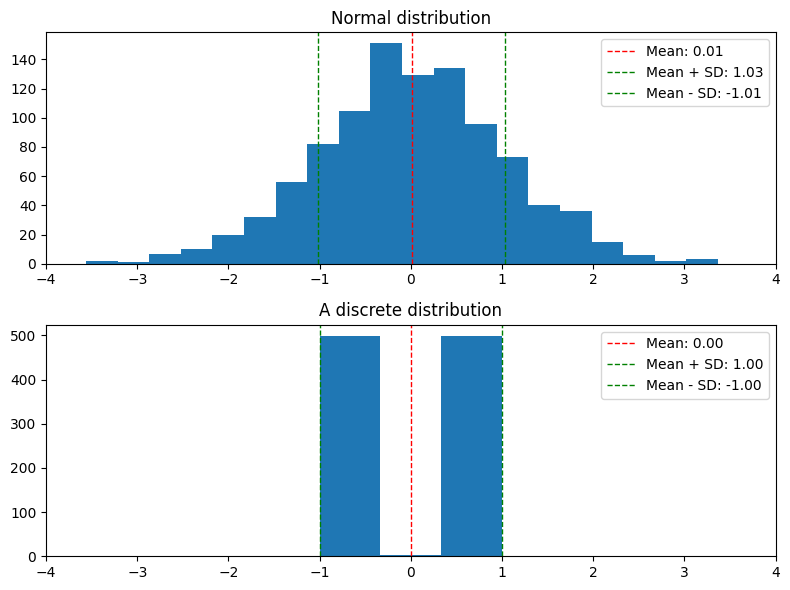
Two different distributions with (almost) the same mean, median, and standard deviation.
Today we study how features of the data can influence summary statistics.
The Mean#
The mean is good#
The mean is one proxy for the “center” of the distribution.
A common tendency is to conflate “center” with “typical value”.
In some cases, this is reasonable.
For example:
Example (Scientific Experiments): You do \(n\) independent experiments to measure the value of a fixed, bounded quantity \(Q\), e.g.:
The average concentration of microplastics in the Palo Alto water supply
The plasticity of a protein
The fraction of students who think a hot dog is a sandwich
Because of natural variation and measurement error, each experiment is a possibly noisy measurement of \(Q\).
In Unit 4, we’ll see that in such an experiment, the mean of our dataset is likely to be very close to \(Q\), as long as \(n\) is large enough.
But many types of data we encounter are not like this!
Misleading means#
Features of a dataset that can “throw off” the mean as a measure of the “typical” value:
Multi-modal data
Skewed and heavy-tailed distributions
Outliers
High variability
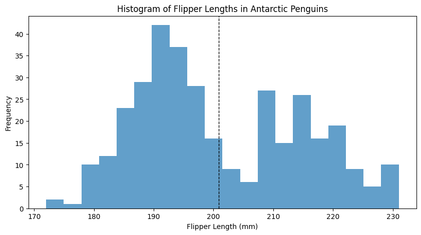
Misleading means 1: multi-modal data#
The mode of a dataset is the value that appears most frequently, or the highest point in the histogram.
Antarctic penguin data from the research of K. Gorman
Sometimes, people use the term more loosely, using “mode” to refer to a “lump” in a histogram.
A common intuition is that that the mean is roughly where the mode is.
In some cases, like the “independent experiments” case, this is true.
But sometimes, a dataset is naturally multi-modal.
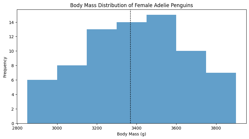
Multi-modal data#
Many datasets can be naturally decomposed into natural subsets.
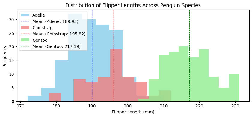
Within each subset, there is only one mode.
In this case, within that subset, the mean and mode do match!
Effects of multiple modes on the mean#
In a multi-modal dataset, the dataset’s mean value lies between the means of the different modes.
In that case, it is not representative of a “typical” sample.
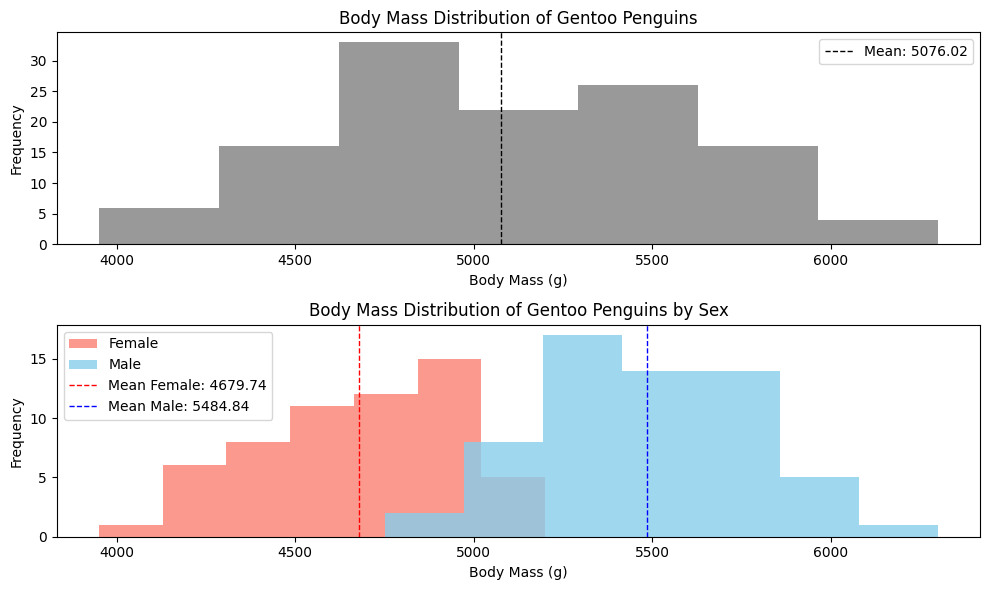
Here, the mean for the entire dataset is on the large end for a female, but on the small end for a male.
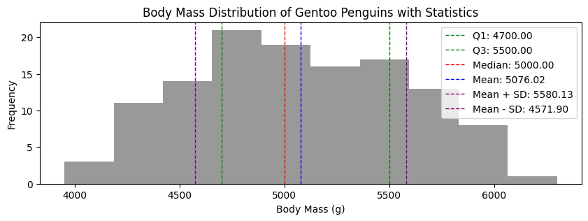
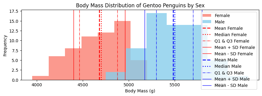
Summary statistics of multi-modal data#
Question: Should the median also be influenced by multiple modes?
Question: Should quantiles be influenced by multiple modes?
Question: Should the standard deviation be influenced by multiple modes?
Yes! In the sense that the aggregate data’s median, quantiles, and standard deviation do not reflect what is going on in the specific modes.
Why does this matter?#
Many times, the mean (and other summary statistics) are used to make decisions.
When decisions are based on statistics of all of the data, instead of mode-by-mode, then it might not be the right decision for everyone.
Here is a synthetic example:
A medical researcher at a hospital records the duration of symptoms for a new disease.
The average amount of time the symptoms are experienced is 20 days.
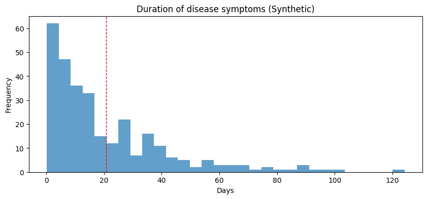
The data does not look obviously multimodal.
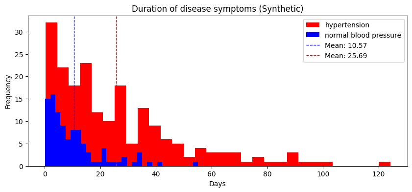
But suppose we separately analyze the data for patients with and without hypertension; in that case, we see that the average duration of symptoms for patients without hypertension is much shorter:
A real example?#
Consider this plot of time-to-onset for COVID symptoms:
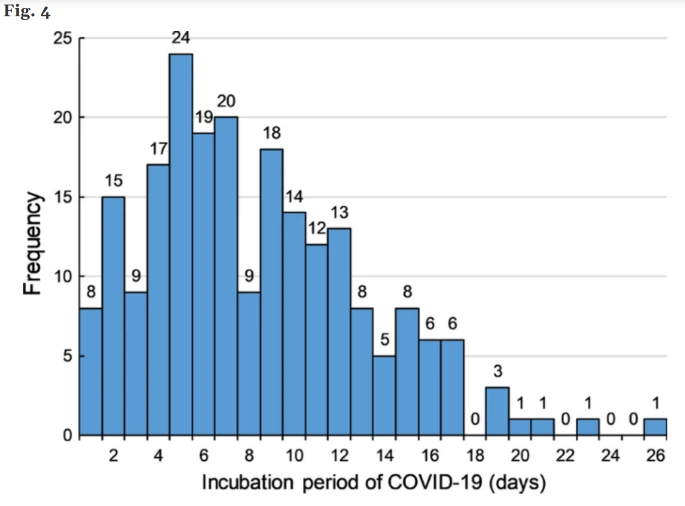
Question: Could this data be multimodal? Suppose we make recommendations for isolation time after close contact based on this data—in what sense is this problematic? What are the tradeoffs that we have to make?
Misleading Means in the Media#
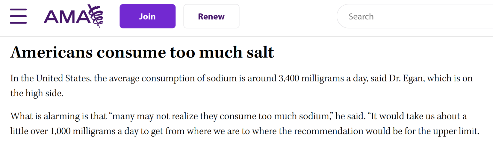
Is this representative of most people? Could the data be multimodal? Is there a lot of variability?
A closer look#
A CDC study suggests that:
The data is multimodal: women consume about 3000 mg per day on average, and men consume about 4000 mg per day on average.
Variability is limited, in the sense that 86.7% of American adults are eating more than the recommended 2300 mg. Note that this leaves open the possibility that all 11% of Californians are eating the recommended amount :P
The conclusion that Americans are eating more salt than the medical community suggests they should is still valid. But the 3400 mg figure is still misleading.
Skew#
Even when the distribution has only one mode, it can be skewed.
Colloquially, this means that the histogram “stretches out” to the left or the right.
There are several quantitative measures of skewness; I don’t expect you to know any of them, only the concept of skew.
Sometimes people also say the distribution is heavy-tailed (because the stretched out part looks like a tail?).
Right-skewed data#
Types of data that tend to be skewed to the right:
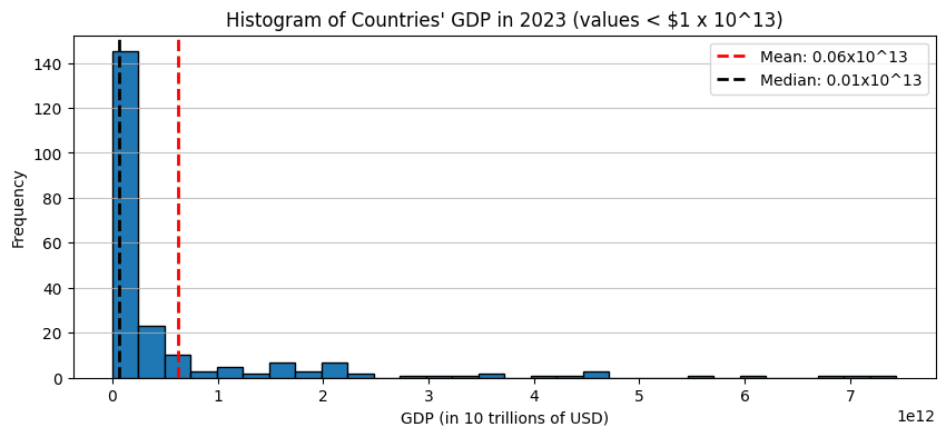
Incomes, GDP, number of awards won, views or clicks online: “the rich get richer”
Waiting times (e.g. time between earthquakes or volcanic eruptions)
Sizes of some natural objects (lakes, rocks, mineral deposits) Also an example of the rich get richer or poor get poorer?
Effect of right skew on the mean#
If a distribution is skewed to the right, then typically the median/mode will be smaller than the mean.
Left-skewed data#
Types of data that tend to be skewed to the left:
Age of mortality
Exam scores
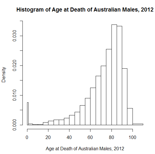
Effects of left skew on the mean#
If a distribution is skewed to the left, then typically the median/mode will be larger than the mean.
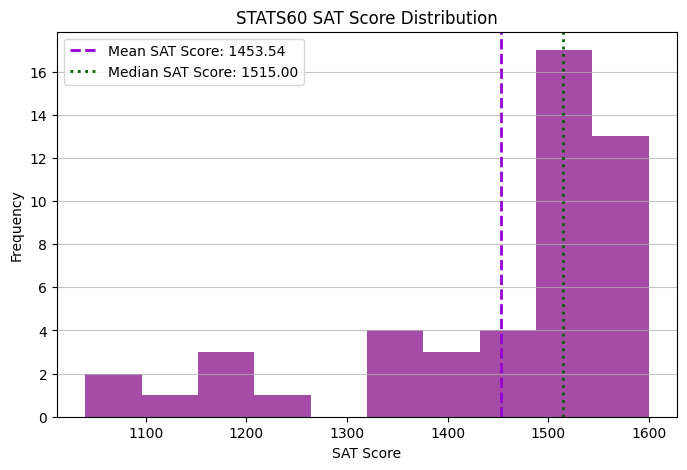
Measuring skewness#
The gap between the mean and the median is one quantitative measure of skew!
Outliers#
Outliers (abnormally large or small values) can move the mean away from the median or mode.
Outliers and skew are related: outliers do skew the distribution.
The distinction is usually that we think of outliers as anomalies, whereas skew can be a “natural” property of the data.
Outliers in social media usage#
This is a histogram of responses to the in-class survey question “How many minutes per day do you spend on social media?”
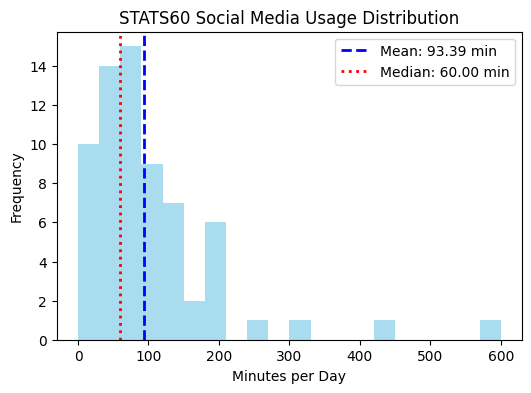
One of you replied \(10\) hours, that is \(600\). This is an outlier.
Statistic |
dataset with outlier |
dataset without outlier |
|---|---|---|
Mean |
93.4 min |
85.7 min |
Standard Deviation |
97.0 min |
74.5 min |
Median |
60 min |
60 min |
High-variability datasets#
If the variability of a dataset is high, then the mean or median is no longer representative of a “typical” sample.
This is a histogram of responses to the course data survey question “How many hours per week do you spend studying?”
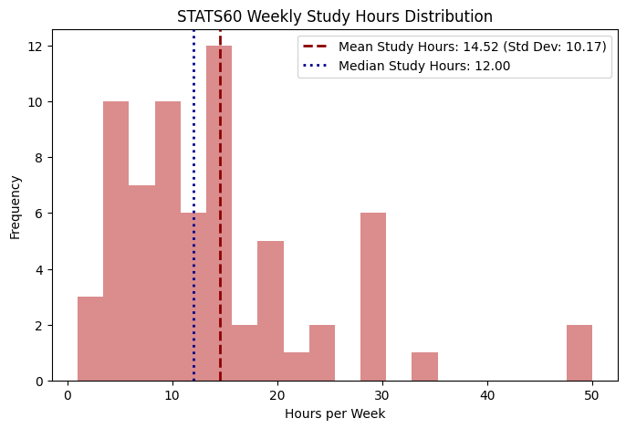
The mean and median are pretty close.
But the variability is really high; in my opinion, neither the mean (14.5 hrs) nor the median (12 hrs) can be taken as representative of a “typical” student.
More high-variability datasets#
Another example of a situation where the mean is not necessarily representative is in gambling:
Flip a fair coin for \(\$300\).
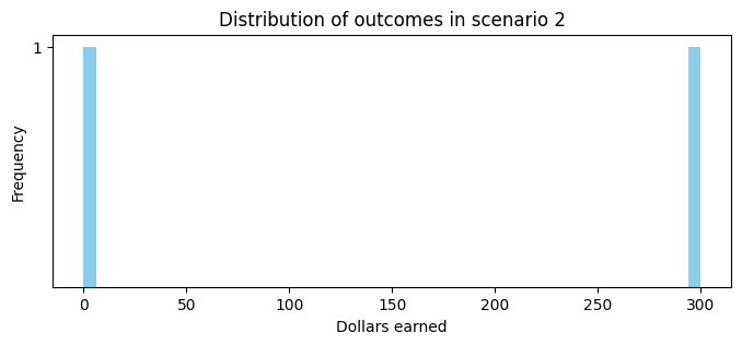
Remember the mean is \(\$150\).
Neither situation is really like the mean.
Standard deviation#
The standard deviation as a measure of variability#
The standard deviation \(\bar{\sigma}\) is a proxy for “average distance to the mean,” \(\bar{x}\).
As discussed briefly on Monday, most datapoints are at most a few standard deviations away from the mean.
By a fact called Chebyshev’s inequality, we know that a \(1-\frac{1}{t^2}\) fraction of datapoints are within \(t\) standard deviations of the mean.
For example, taking \(t = 2\), we know that at least \(75\%\) of datapoints are within \(2\) standard deviations of the mean.
Standard deviation can overestimate variability#
We know for sure that \(\ge 75\%\) of \(x_i\) are in the window \((\bar{x} - 2\sigma, \bar{x} + 2\sigma)\).
Many times this is a dramatic overestimate!
In the plots below, almost 90% of the data is within 2 standard deviations of the mean! About 65% of the data is within 1 standard deviation of the mean.
In this case, the standard deviation is, qualitatively, an overestimate of the variability.
Outliers and the standard deviation#
Outliers and heavy tails can make the standard deviation really large.
Example: The following dataset gives section attendance for each of the 5 sections of STATS60 this week:
TA |
Attendance |
|---|---|
Cole |
20 |
Junyi |
6 |
Leda |
27 |
Skyler |
25 |
Valerie |
21 |
The mean is 19.8, the standard deviation is 7.3.
If we remove the outlier of Junyi’s section:
the mean is 23.3, the standard deviation is only 2.9.
Outliers and the standard deviation#
One of you replied \(10\) hours, that is \(600\). This is an outlier.
Statistic |
dataset with outlier |
dataset without outlier |
|---|---|---|
Mean |
93.4 min |
85.7 min |
Standard Deviation |
97.0 min |
74.5 min |
Median |
60 min |
60 min |
A robust measure of variability#
Question: what should we use as an alternative measurement of variability?
Quantile widths are more robust to outliers.
Recap#
Summary statistics are just a snapshot.
Different distributions can have the same summary statistics.
The mean and standard deviation behave differently than we expect if the data has
Multi-modality
Skewness
Outliers
What does this mean for us?
The bottom line is that any summary statistic is just a summary; often useful, but sometimes incomplete. You have to look at the data to be sure.