Lecture 21: Testing for Correlation#
STATS 60 / STATS 160 / PSYCH 10
Concepts and Learning Goals:
Hypothesis test for correlation coefficients
testing via simulation
permutation test
Variability of the correlation coefficient
via simulation! “the bootstrap”
Taking inventory#
Suppose we have conducted an experiment and we have used our data to compute a summary statistic, \(\hat{T}\).
We suspect that \(\hat{T}\) is indicative of a trend. But it could just be random noise…
Example 1: a student takes a 10-question True/False test, and \(\hat{T} = 8/10\) is the fraction answered correctly.
It seems like the student knows the material!
Is it possible they were just guessing randomly?
Example 2: we run a randomized controlled trial to see if retrieval practice helps students study, and \(\hat{T} = -1\) is the difference in mean scores between the treatment and control group.
It seems like retrieval practice is worse for remembering the material!
Is a \(-1\) difference in average score really a lot? Could it just be noise?
Question:
Explain what a hypothesis test is, and why we would do it, in plain English, using 25 words or less.
Explain what a null hypothesis is in plain English, using 25 words or less.
Explain what a \(p\)-value is in plain English, using 25 words or less.
Hypothesis testing recap#
Suppose we have conducted an experiment and we have used our data to compute a summary statistic, \(\hat{T}\).
We suspect that \(\hat{T}\) is indicative of a trend. But it could just be random noise…
A hypothesis test is a thought experiment to help us figure out whether it is likely that our observation \(\hat{T}\) is just random noise.
The null hypothesis is that our data is just random, with no trend.
The specifics of the null hypothesis depend on the experiment we ran.
The p-value is the chance of observing \(\hat{T}\) or an even stronger trend under the null hypothesis, if the data were random.
Correlation#
Suppose that I have sampled \(n\) individuals from my population, and for each I have measured the values \((x_i,y_i)\).
For example:
Penguins: \(x =\) body mass, \(y=\) beak length
Health: \(x=\) weight, \(y=\) breakfast days/week
Economics: \(x=\) years of education, \(y=\) salary
College admissions: \(x=\) SAT score, \(y=\) sophomore-year GPA
The correlation coefficient (\(R\)) of \(x\) and \(y\) is the slope of the best-fit line for the standardized datasets \(x_1,\ldots,x_n\) and \(y_1,\ldots,y_n\).

Do students who study more sleep more?#
Let’s look at some data from the course survey. Here is a scatterplot of your self-reported “hours of sleep” vs. “hours of studying:
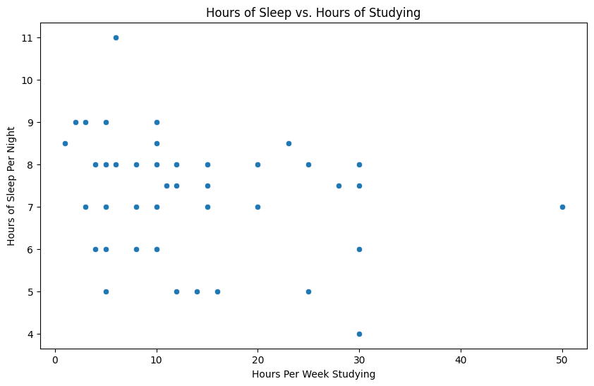
Does it look to you like there is a positive association, negative association, or neither?
Correlation coefficient for sleep vs. study#
Here is the best-fit line. \(R = -.19\).
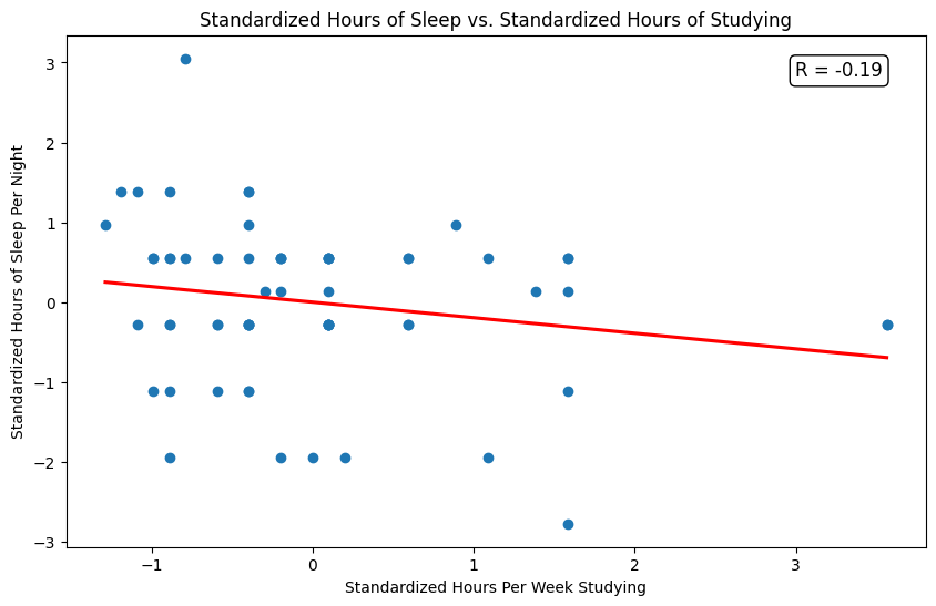
Is this a real trend or is it just noise?
Is this a significant correlation?#
How can we decide if the correlation coefficient \(R\) is large? How can we decide if it significant?
To decide if \(R\) is large: compare to its max/minvalues, \(1\) and \(-1\).
But \(R\) can be significant (a real linear association) even when \(|R|\) is smaller than 1.

Testing for correlation#
Suppose that we compute the correlation coefficient, and see that it has value \(R \neq 0\).
Is this just a coincidence? Or is the correlation a real pattern?
Let’s formulate this as a hypothesis testing problem:
Null Hypothesis: there is no correlation.
How can we compute the \(p\)-value?
We’ll use simulation!
Permuting the datapoints#
Let’s assume, from now on, that our \(x_i\) and \(y_i\) are standardized.
Suppose there really is a positive association between \((x_i,y_i)\).
Now, what if we randomly shuffle or permute the \(y_i\), so that they are matched to a random \(x_j\)?
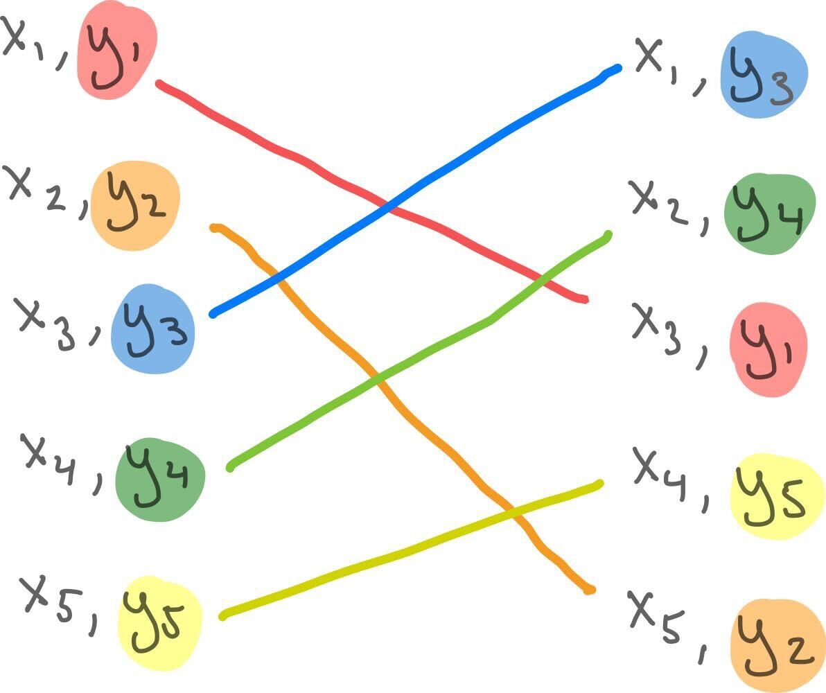
There’s almost certainly no correlation now!
Null hypothesis based on shuffling#
Suppose we have computed \(R\) from our data.
We want to know if \(R\) reflects an actual trend, or if it is just noise.
Null hypothesis: the pairs \((x_i,y_i)\) are paired up totally randomly.
Question: Why is this null hypothesis saying that there is no real correlation?
Question: In plain English, what is the \(p\)-value of \(R\) for this null hypothesis?
The null is saying there is no real correlation because if the pairing of \(x_i\) and \(y_i\) is arbitrary/random, there would almost certainly not be a linear relationship (as long as \(n > 2\), two points always make a line!).
The \(p\)-value is the chance that you’d get this value of \(R\), or a more extreme one, if the data were paired up by randomly shuffling.
Permutation test for correlation#
Suppose we have computed \(R\) from our data.
We want to know if \(\hat R\) reflects an actual trend, or if it is just noise.
Null hypothesis: the pairs \((x_i,y_i)\) are paired up totally randomly.
\(p\)-value: the chance that you’d get this value of \(R\), or a more extreme one, if the data were paired up by randomly shuffling.
We’ll compute the \(p\)-value using a Permutation test, a test based on simulation:
Do some large number \(T\) of repetitions of the following experiment:
a. Randomly permute/shuffle the \(y_i\) so that each is paired with some random \(x_j\)
b. Compute and record the correlation coefficient for the shuffled dataset
Make a histogram of the correlation coefficient values for all \(T\) trials.
Decide the \(p\)-value for \(R\) based on how extreme it is relative to the histogram:
If \(R\) is positive, the \(p\)-value for \(R\) is the fraction of histogram values larger than \(R\) (or \(1/T\), if none are larger).
If \(R\) is negative, the \(p\)-value for \(R\) is the fraction of histogram values smaller than \(R\) (or \(1/T\), if none are smaller).
The penguins#
In our correlation lecture, we computed a correlation coefficient of \(\hat R = 0.67\) for Gentoo Penguin body mass vs. beak length.
What is the \(p\)-value?
Permutation test for penguin correlation#
I ran a simulation with \(T = 10,000\) trials.
In each trial, I chose a new random permutation of the \(y_i\), and computed the correlation coefficient.
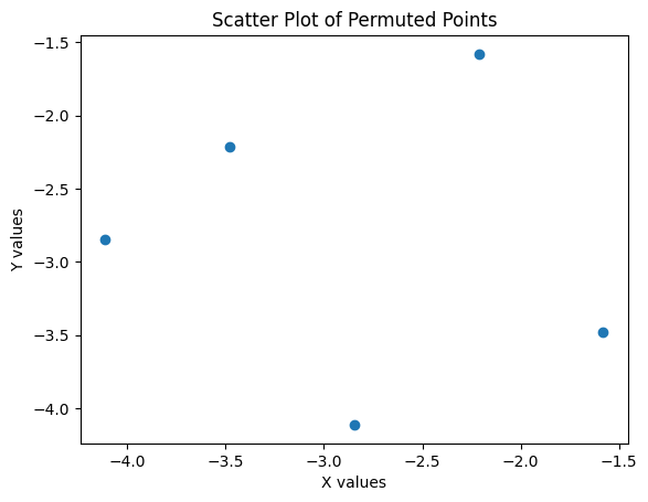
Here is trial 1:

Here is trial 2:

Etc.
Aggregating the trials#
Below is a histogram of the dataset of the correlation coefficients from each of the \(T\) trials.

Using the permutation test, the \(p\)-value is at most \(.0001\):
We conclude that \(R\) is statistically significant at level \(\alpha = 0.05\) (or smaller).
GDP in 1960 vs. 2000#
In the correlation lecture we also computed the correlation coefficient for the GDP of countries in 1960 vs. 2000.

We can do a permutation test to check if this value of \(R\) is statistically significant.
P-value for GDP correlation#
For \(T = 10,000\) permutations, the \(p\)-value is for the correlation coefficient of 1960 vs. 2000 GDP is \(1/10,000\):

Back to sleep vs. study#
Let’s return to our course survey data, about hours of sleep vs. hours of study.
We calculated \(R = -.19\) for this data. Is it significant?
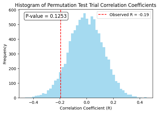
P-value for sleep vs. study#
Via simulation, for a \(T = 10,000\)-trial permutation test, we verify that the \(p\)-value is \(\approx 0.13\), so the trend is not statistically significant at level \(\alpha = .05\).
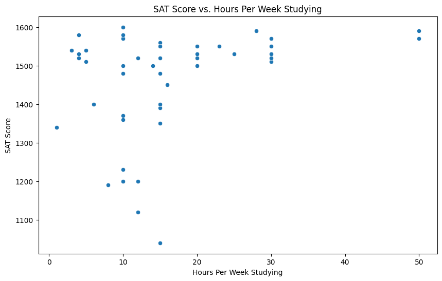
SAT score vs. study#
Let’s look at a different correlation in our course survey dataset: SAT score vs. average number of hours a week spent studying.
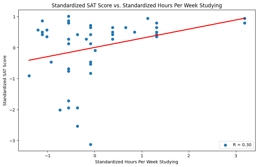
Correlation coefficient for SAT score vs. study#
The correlation coefficient is positive (unsurprisingly?), \(R = .3\)
Statistically significant?#
Again we do \(T = 10,000\) permutation tests:
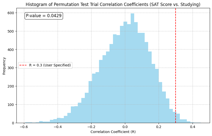
Statistically significant at level \(\alpha = 0.05\)!
Variability#
We computed \(R\) for our data. But what about its variability?
Is \(R\) being influenced by outliers?
If our data had been sampled a bit differently, would my value of \(R\) be dramatically different?
The permutation-test \(p\)-values only give us a sense of statistical significance of a correlation:
we can see how extreme \(R\) is relative to a random shuffling of the data (no correlation)
we cannot see how \(R\) would vary if we had a different sample from data with the same type of associative relationship.
How much variability in SAT score vs. study?#
The SAT score vs. study trend:
Would the value of \(R\) changed to a (smaller or larger) negative value if we had sampled differently? There appear to be some outliers.
How much smaller or larger?
Estimating variability with simulation#
We can use simulation to estimate variability too.
The best case scenario would be, if we have access to new samples from our population, just collect more samples and compute a fresh correlation coefficient a bunch of times.
But what if we don’t have access to new samples?
The following approach is called the bootstrap:
Start with our dataset \((x_1,y_1),\ldots,(x_n,y_n)\).
For some large number of trials \(T\):
a. Sample \(n\) pairs independently with replacement from the dataset: $\((x_{i_1},y_{i_1}),\ldots,(x_{i_n},y_{i_n})\)$
b. Compute and record the correlation coefficient of these pairs.
Form a histogram of the correlation coefficients from all \(T\) trials.
The Bootstrap#
To get a sense of the variability of \(R\):
Start with our dataset \((x_1,y_1),\ldots,(x_n,y_n)\).
For some large number of trials \(T\):
a. Sample \(n\) pairs independently with replacement from the dataset: $\((x_{i_1},y_{i_1}),\ldots,(x_{i_n},y_{i_n})\)$
b. Compute and record the correlation coefficient of these pairs.
Form a histogram of the correlation coefficients from all \(T\) trials.
Question: why could this simulation give us a good sense of variability? Will it account for outliers?
There’s a reasonable chance that we’ll avoid any specific outlier in a trial when we sample with replacement: $\(\Pr[\text{avoid i }] = (1-\frac{1}{n})^n \approx e^{-1} \approx \frac{1}{3} \text{ when }n\text{ large.}\)$
Question: will this always give us a good idea of the variability of \(R\)?
Not necessarily; our sample could just be really weird.
Simulation for variability in sat vs. study#
If we do a bootstrap simulation with \(T= 10,000\) trials, we can see that the confidence interval around \(R\) is actually quite small:
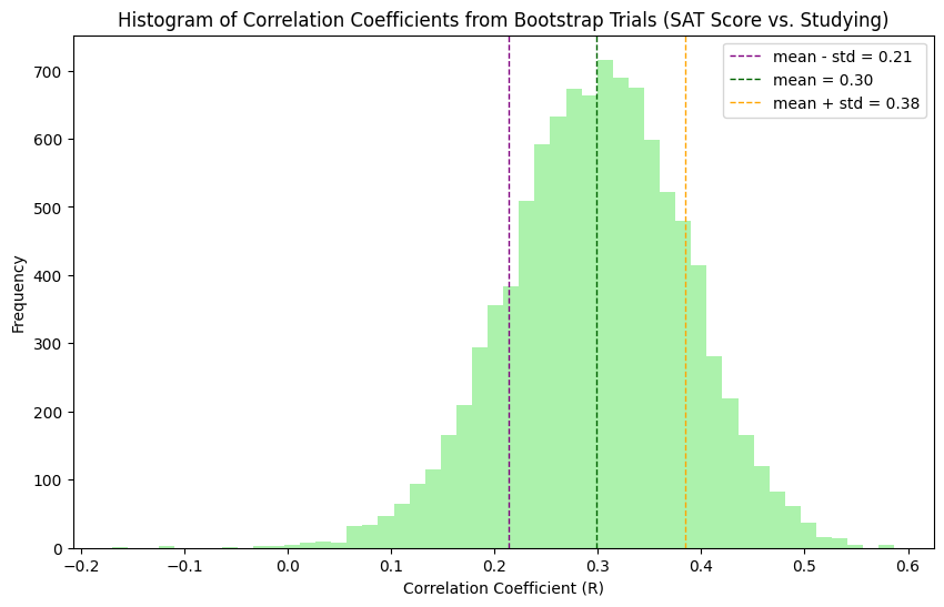
This gives us some sense of the variability of \(R\).
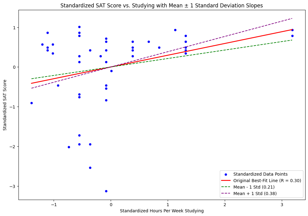
Variability of the best-fit line#
Here you can see the original scatterplot and best-fit line, with the lines corresponding to the mean +/- a standard deviation
The line doesn’t too change much! Variability of \(R\) is reasonably low.
Recap#
Testing for correlation
Using simulation: permutation tests
Variability of correlation
Using simulation: “the bootstrap”