Alternative two sample#
Download#
Kernelizing Hotelling \(T^2\)#
library(pdfCluster)
data(oliveoil)
# let's make it a two-sample dataset (of 3 regions)
X = oliveoil[oliveoil$macro.area %in% c('South', 'Centre.North'),]
#| echo: true
South = X[X$macro.area=='South',3:10]
North = X[X$macro.area=='Centre.North',3:10]
X_1 = as.matrix(South)
X_2 = as.matrix(North)
pdfCluster 1.0-4
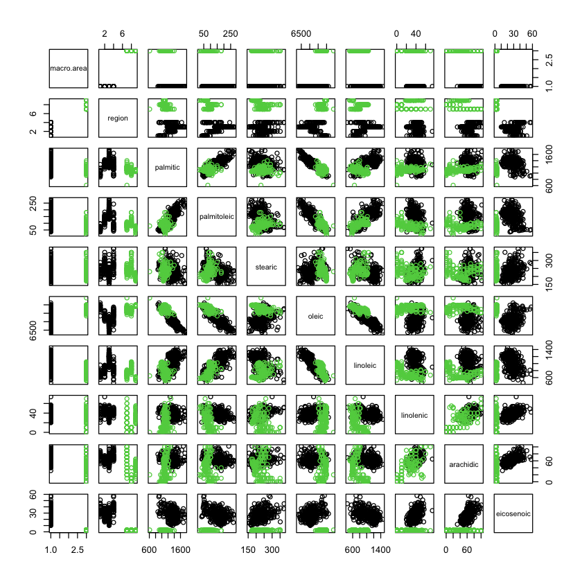
Olive oil data South vs Centre.North#
pairs(X, col=X$macro.area)
Gram matrices#
We used the term Gram matrix last time for a reason.
For any covariance kernel \(K:\mathbb{R}^p \times \mathbb{R}^p \rightarrow \mathbb{R}\) we could use
Gram matrices can be computed for data that is not even Euclidean…
Rearranging a little
with
The other term is
Where does \(W_2\) come from?#
Let \(K(x,y)=x^Ty\) be the linear kernel. Then,
This last term should be subtracted to get an unbiased estimate of \(\|E_{F_1}(X)-E_{F_2}(X)\|^2_2\).
We see then, that for any feature map \(h:\mathbb{R}^p \rightarrow \mathbb{R}^k\) leading to kernel \(K(x,y)=h(x)^Th(y)\) subtracting this \(W_2\) term yields unbiased estimate of
Maximum Mean Discrepancy Statistic (MMDS)#
When \(K\) is the Gram matrix of a covariance kernel, Gretton et al. (almost) propose \(W_1(G)\) as a two-sample test.
Specifically they propose (up to scaling)
MMDS in general#
For a class of functions \({\cal F}\) define $\( MMD({\cal F}; F_1, F_2) = \sup_{h \in {\cal F}} E_{F_1}(h(X)) - E_{F_2}(h(X)) \)$
When \({\cal H}\) is the unit ball in an RKHS with kernel \(K\) they show $\( MMD({\cal H}; F_1, F_2) = E_{F_1 \times F_1}(K(X,X')) + E_{F_2 \times F_2}(K(X,X')) - 2 E_{F_1 \times F_2}(K(X,X')) \)$
Notation: \(E_{F \times G}[h(X,X')]\) denotes expectation under \((X,X') \sim F \times G\).
Statistic of Gretton et al. is an estimator of \(MMD({\cal H}; F_1, F_2)\).
Using kernel property, it is not hard to see that the analog of (rescaled) \(\text{Tr}(XX^TP^{\Delta})\) is given by
Like \(\widehat{MMD}({\cal H}; X_1, X_2)\) but includes this \(W_2\) term…
kernlab#
#| echo: true
library(kernlab)
kmmd(X_1, X_2)
Using automatic sigma estimation (sigest) for RBF or laplace kernel
Kernel Maximum Mean Discrepancy object of class "kmmd"

Gaussian Radial Basis kernel function.
 Hyperparameter : sigma =  2.8390782080874e-06


 H0 Hypothesis rejected :  TRUE
 Rademacher bound :  0.444461696552373

 1st and 3rd order MMD Statistics :  0.901532029840108 0.643725854362546
#| echo: true
kmmd(X_1, X_2, kernel='vanilladot', kpar=list())
Kernel Maximum Mean Discrepancy object of class "kmmd"

Linear (vanilla) kernel function.


 H0 Hypothesis rejected :  FALSE
 Rademacher bound :  3760.42987748469

 1st and 3rd order MMD Statistics :  798.276202069945 399126.145253863
Energy statistics#
Energy statistics#
We saw that Hotelling’s \(T^2\) test is essentially determined by an \(n \times n\) (case) similarity matrix \(G\):
A simple way to construct a similarity matrix is from a distance matrix \(D_{ij} = d(X_i, X_j)\) and setting
Noting that \(\text{Tr}(P^{\Delta}) = 1\) suggests simply using
These are the energy test statistics of Szekely et al..
Permutations can be used to get valid tests (in package
energyinR)
Energy test with Euclidean distance#
#| echo: true
library(energy)
X = rbind(X_1, X_2)
n_1 = nrow(X_1)
n_2 = nrow(X_2)
D = dist(X)
T = eqdist.etest(D, c(n_1, n_2), distance=TRUE, R=500)
T
	2-sample E-test of equal distributions

data:  sample sizes 323 151, replicates 500
E-statistic = 94382, p-value = 0.001996
Sanity check#
#| echo: true
M_1 = c(rep(1, n_1), rep(0, n_2)) / n_1
M_2 = c(rep(0, n_1), rep(1, n_2)) / n_2
P_delta = (M_1 - M_2) %*% t(M_1 - M_2) * n_1 * n_2 / (n_1 + n_2)
Dm = as.matrix(D)
c(package.value=T$statistic, byhand=-sum(diag(P_delta %*% Dm)))
- package.value.E-statistic
- 94382.2812754321
- byhand
- 94382.2812754317
Classification two-sample tests (C2ST)#
LDA classifier#
A natural classifier related to our two sample problem is to map a new test point \(x\) to the class \(i\) that (under equal sample sizes) minimizes
For test data \(H_0:F_1=F_2\), such a classifier should be roughly a coin flip.
This is the basis of the C2ST
General procedure#
Create label $\( Y = \begin{pmatrix} 1_{n_1} \\ 2_{n_2} \end{pmatrix} \)$ and form
D=cbind(Y, X)Split
Drandomly up in toD_testandD_trainin such a way that for test data the number of cases fromX_1matches that ofX_2. Letn_testdenote the total number of cases of each held out.Fit a classifier \(\hat{C}\) on
cbind(X_train, Y_train), and evaluate its classification accuracy oncbind(X_test, Y_test).Under \(H_0:F_1=F_2\), conditional on
D_trainthe accuracy has (approximate) distribution $\( \frac{1}{n_{test}} \text{Binomial}\left(n_{test}, \frac{1}{2} \right). \)\( (This seems easiest to justify when \)X_i\( are simple random samples from large populations -- in this case given case \)x$ is selected a Bernoulli(1/2) determines which sample it finds itself in.)
References#
Section 3.6 of Mardia, Kent and Bibby
DISCO analysis: A nonparametric extension of analysis of variance
Comments#
This is almost \(W_1(G;X_1,X_2)\): if \(K\) is bounded by \(C'\), difference is bounded by \(C'/n\).
Easy to analyze their form as it is exactly a two-sample \(U\) statistic (degenerate under \(H_0\)).