Covariance models#
Download#
Graphical LASSO#
A different model for covariances: models \(\Theta=\Sigma^{-1}\).
Problem is
where \(\|\cdot\|^-_1\) does not penalize diagonal part of \(\Theta\).
As we have a likelihood we can in principle use cross-validation to choose \(\lambda\).
What’s the point?#
Graphical models#

Graphical models (can) encode conditional independences.
In Gaussian models these are represented by
0in \(\Sigma^{-1}\)
Example#
Multivariate normal#
Figure (a) represents \(X \perp Z | Y\)
Implies that \(\Sigma_{XZ}=0\).
Formally if \(W \sim N(0, \Theta^{-1})\) and \(\Theta_{ij}=0\) then \(W_i \perp W_j | W_{-\{i,j\}}\).
Relation to log-linear models#
Suppose \(X, Y, Z\) were discrete variables and \(N\) is a contingency table with axes
X,Y,Z.The above conditional independence can be encoded as
glm(N ~ X + Y + Z + X:Y + Y:Z, family=poisson)
Limiting interactions to 2nd order, any undirected graph can be converted to such a model.
Figure (d) is the model
glm(N ~ X + Y + Z + W + X:Y + Y:Z + Z:W, family=poisson)
Back to graphical LASSO#
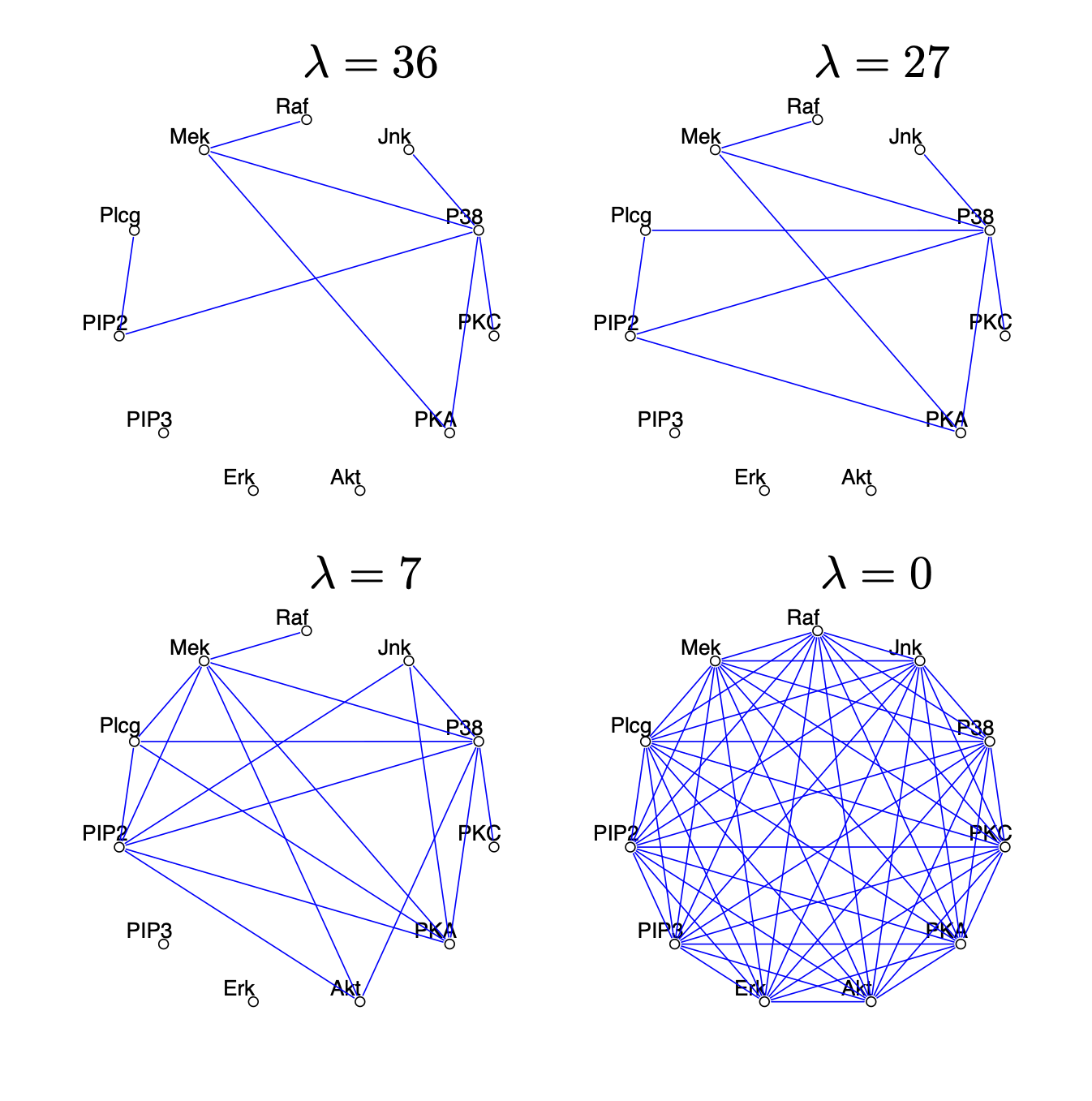
Choosing \(\lambda\) sets the sparsity level.
The graphical LASSO tries to make decisions about all \(\binom{p}{2}\) conditional independencies simultaneously.
Fitting graphical LASSO#
If \(p\) grows, then directly using the likelihood becomes expensive (gradients is \(O(p^3)\) for inverting \(p \times p\))…
Graphical LASSO algorithm solves by iterative LASSO solves…
Graphical LASSO#
#| echo: true
library(glasso)
flow = read.table('http://www.stanford.edu/class/stats305c/data/sachs.data', sep=' ', header=FALSE)
G = glasso(var(flow)/1000, 27)
library(corrplot)
Theta = G$wi
Theta = Theta / outer(sqrt(diag(Theta)), sqrt(diag(Theta)))
corrplot(Theta, method='square')
corrplot 0.95 loaded

Using sklearn#
CV curve#
Best estimator#
Alternative approaches#
Meinshausen and Buhlmann (2006) use the fact that (for centered \(X\))
Further,
Therefore, \(\theta_j[k] = 0 \iff \Theta_{jk}=0\) \(\implies\) conditional independencies of interest can be learned by regressions
lm(X[,j] ~ X[,-j])
Can induce sparsity by
glmnet(X[,-j], X[,j])
Combining edge sets#
One downside to this approach is that we make two decisions about \(X_j \perp X_k | X_{-\{j,k\}}\):
Once when response is \(X[,j]\), the other when the response is \(X[,k]\).
Solutions#
Make a decision using
ANDorOR…
Or#
Maybe, we could we tie the parameters together in the \(p\) different LASSO problems?
This is essentially pseudo-likelihood (more shortly)
Combining factor analysis and low-rank#
We finished Factor Analysis section off with a convex relaxation of factor analysis / low-rank
Can combine this with graphical LASSO
Extension to mixed data#
What if \(X \in \mathbb{R}^p\) is continuous but \(Y \in \{1,2,3,...,L\}\) discrete?
What is the analog of
glm(N ~ X + Y + X:Y, family=poisson)
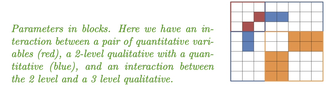
2nd-order potentials (first order interactions in log-linear models)#
Natural analog (with \((y_1,\dots, y_L)\) a one-hot encoding) considered by Lee and Hastie (2012)
Can have multiple discrete variables as well (with a single variable the above model is LDA - linear discriminant analysis)
Mixed graphical models#
Fitting mixed models#
For
glassothere is an explicit likelihood to maximize, but mixed models will have some awful intractable normalizing constant…BUT for each variable, our modeling choices have nice conditional likelihoods.
For continuous variables \(X_i\) is Gaussian with mean and covariance determined by \(\Theta\).
Discrete variables \(Y_j\) are multinomial with specific multinomial logistic models determined by \(\Theta\)
(Penalized) pseudo-likelihood#
Often, \({\cal P}\) will separate over variables but the individual likelihoods tie parts of \(\Theta\) together…
Pseudo-likelihood#
Consider a simple Ising model: i.e. a binary random vector \(B \in \{0,1\}^J\) with mass function
Matrix \(A\) an adjacency matrix for some graph.
The normalizing constant requires summing over \(2^J\) states…
Conditional likelihoods#
For any \(j\),
This conditional has a simple normalizing constant
Summing log over \(j=1, \dots, J\) yields an expression that’s simple to optimize
Working in this model, at “true” parameters \((c_1^*, c_2^*)\) we have the gradient of the pseudo-likelihood is centered (just like the likelihood).
Yet another model for covariance: additive#
We’ve considered two general models for covariance so far:
Diagonal + Low-Rank (PPCA & Factor Analysis)
Sparse precision (Graphical LASSO)
Combination of the two…
Additive model#
Given \(C_j \succeq 0, 1 \leq j \leq k\)
Generative model#
EM for additive model#
Complete (negative) log-likelihood#
E-step#
Given current \(\alpha_{\text{cur}}=\alpha_c\) we need to compute
\(M\)-step#
A generalization#
Given \(D_j, 1 \leq j \leq k\)
Could impose structure on \(\bar{\Sigma}_j\) (e.g. diagonal, \(c \cdot I\), etc)
This is (stylized) version of RFX covariance
Generative model#
EM for RFX model#
Complete (negative) log-likelihood (\(n=1\))#
E-step#
Given current estimates \(\bar{\Sigma}_c=(\bar{\Sigma}_{j,c}, 1 \leq j \leq k)\), we need to compute
M-step#
Unrestricted MLE having observed \(\mathbb{E}_{\bar{\Sigma}_c} [Z_jZ_j'|X]\)…
More realistic RFX setup#
Generative model#
Switching to errors notation \(\epsilon\)…
Some of the \(Z_{ij}\)’s will be of different sizes (depending on how many observations subject \(i\) contributes…)
Complete (negative) log-likelihood#
Need to compute
An example in a little more detail#
Repeated measures#
For subject \(i\) with \(n_i\) measurements $\( \begin{aligned} \alpha_i &\sim N(0, \sigma^2_R) \\ \epsilon_{i} & \sim N(0, \sigma^2_M \cdot I) \\ X_{i} &= \alpha_i 1_{n_i} + \epsilon_{i} \end{aligned} \)$
\(\implies\) contribution of subject \(i\) to complete (negative) log-likelihood is
Total covariance is \(\sigma^2_R C_R + \sigma^2_M \cdot I\) with \(C_R\) block diagonal
M-step \(\sigma^2_R\)#
Given \(\theta_c = (\sigma^2_{M,c}, \sigma^2_{R,c})\):
Sherman-Morrison-Woodbury simplifies above expression, leads to closed-form update \(\sigma^2_{R,u}\)
ECM performs blockwise updates to parameters… does not fully maximize before subsequent E-step
M-step \(\sigma^2_M\)#
Given partially updated \(\theta_{c+1/2} = (\sigma^2_{M,c}, \sigma^2_{R,u})\):
This is ECM, Meng and Rubin (1993).
Usefulness of the approach a little more obvious in the presence of mean parameters:
Fix \((\sigma^2_M, \sigma^2_R)\) and estimate \(\beta\),
Fix \(\beta\) and estimate \((\sigma^2_M, \sigma^2_R)\).
ECME#
For any block of \(\theta\), can use the (conditional / blockwise) MLE
For update of \(\sigma^2_M\), fixing \(\sigma^2_R=\sigma^2_{R,u}\) compute
Both ECM and ECME share EM’s ascent property…
Wrapping up#
We’ve discussed several models of covariance…
While not difficult to describe, only some are relatively easy to use in
R:prcompdoppcafactanalglassolme4(for RFX, not discussed here)
Would be nice to have all of these methods easily available in code…
PCA gets used a lot, at least partly because it’s implementation is so simple…
We saw that
sklearnhas some decent implementations of PCA / FactorAnalysis / Graphical LASSOWould being a Bayesian make life easier?