PCA I#
Download#
PCA#
Two views#
Low-rank matrix approximation
Maximal variance projection
Low-rank approximation#
Consider problem
with
This is reduced rank regression objective with \(\tilde{Y}=R_cX\), \(\tilde{X}=I\), \(\Sigma=I\).
Going forward, we’ll somtimes drop \(R_c\) by assuming that \(R_cX=X\), i.e. that it has already been centered.
Solution#
Our reduced-rank regression solution told us to look at \(\tilde{W}\), \(k\) leading eigenvectors of
Then, we take
Relation to SVD#
Given matrix \(M \in \mathbb{R}^{n \times p}\) (assume \(n>p\)) there exists an SVD
Properties#
Consider
Eigen-decomposition of \(MM^T\) can be found from SVD of \(M\).
Similarly
Finally,
Can absorb \(D\) into \(U\) by writing
Back to reduced rank#
Our reduced rank solution with \(X=UDV^T\) picks
More common to think of rank-\(k\) PCA in terms of first \(k\) scores
and loadings
A second motivation#
Could also consider the problem
Also a reduced rank problem whose solutions are projections onto a k-leading eigenspace of \((X^TX)\).
This one clearly isn’t a likelihood – \(X\) appears as response and design.
Maximal variance#
Minimizing first over \(A\), we see this is equivalent to solving this problem
where \(P_k\) is a projection matrix of rank \(k\).
Equivalently, we solve (recall \(R_cX=X\))
This is the same as

Rank \(k\) PCA captures \(k\) dimensional subspace of features that maximizes variance…
Population version#
The maximizing variance picture lends itself to a population version
Thinking of rows of \(X\) as IID with law \(F\), let \(\Sigma = \text{Var}_F(X[1,])\)
Solution is to choose top \(k\) eigen-subspace of \(\Sigma\)…
PCA = SVD#
Given data matrix \(X \in \mathbb{R}^{n \times p}\) with rows \(X[i,] \overset{IID}{\sim} F\), the sample PCA can be described by the SVD of \(R_cX\)
As \(V\) can be thought as an estimate of \(\Gamma\) in an SVD of
we might write \(V = \widehat{\Gamma}\).
Columns of \(\widehat{\Gamma}\) are the loadings of the principal components while columns of \(UD = \hat{Z}\) are the (sample) principal components scores.
Scaling#
Common to scale columns of \(X\) to have standard deviation 1.
In this case, we are really computing the PCA of
Scalings are
Synthetic example#
#| echo: true
n = 50
p = 10
X = matrix(rnorm(n*p), n, p)
R_c = diag(rep(1, n)) - matrix(1, n, n) / n
SVD_X = svd(R_c %*% X)
Z = SVD_X$u %*% diag(SVD_X$d)
Gamma_hat = SVD_X$v
pca_X = prcomp(X, center=TRUE, scale.=FALSE)
names(pca_X)
- 'sdev'
- 'rotation'
- 'center'
- 'scale'
- 'x'
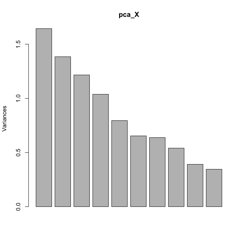
Screeplot: is there an elbow?#
plot(pca_X) # Screeplot
c(varZ2=var(Z[,2]))
Check loadings#
summary(lm(Gamma_hat[,1] ~ pca_X$rotation[,1]))
Warning message in summary.lm(lm(Gamma_hat[, 1] ~ pca_X$rotation[, 1])):
“essentially perfect fit: summary may be unreliable”
Call:
lm(formula = Gamma_hat[, 1] ~ pca_X$rotation[, 1])

Residuals:
       Min         1Q     Median         3Q        Max
-4.787e-16 -1.601e-16  6.330e-18  1.643e-16  5.433e-16

Coefficients:
                     Estimate Std. Error   t value Pr(>|t|)
(Intercept)         3.294e-17  1.049e-16 3.140e-01    0.762
pca_X$rotation[, 1] 1.000e+00  3.317e-16 3.015e+15   <2e-16 ***
---
Signif. codes:  0 ‘***’ 0.001 ‘**’ 0.01 ‘*’ 0.05 ‘.’ 0.1 ‘ ’ 1

Residual standard error: 3.258e-16 on 8 degrees of freedom
Multiple R-squared:      1,	Adjusted R-squared:      1
F-statistic: 9.089e+30 on 1 and 8 DF,  p-value: < 2.2e-16
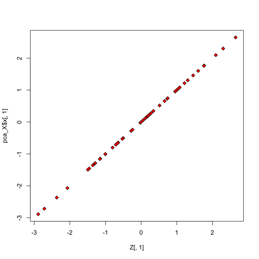
Check scores#
plot(Z[,1], pca_X$x[,1], pch=23, bg='red')
With scaling#
#| echo: true
S_inv = 1/ (sqrt(diag(t(X) %*% R_c %*% X) / 49))
SVD_Xs = svd(R_c %*% X %*% diag(S_inv))
Z_s = SVD_Xs$u %*% diag(SVD_Xs$d)
Gamma_hat_s = SVD_Xs$v
pca_Xs = prcomp(X, center=TRUE, scale.=TRUE)
Check loadings#
#| echo: true
summary(lm(Gamma_hat_s[,1] ~ pca_Xs$rotation[,1]))
Call:
lm(formula = Gamma_hat_s[, 1] ~ pca_Xs$rotation[, 1])

Residuals:
       Min         1Q     Median         3Q        Max
-4.321e-16 -2.714e-16 -2.976e-17  2.422e-16  5.693e-16

Coefficients:
                      Estimate Std. Error   t value Pr(>|t|)
(Intercept)          1.347e-16  1.150e-16 1.171e+00    0.275
pca_Xs$rotation[, 1] 1.000e+00  3.638e-16 2.749e+15   <2e-16 ***
---
Signif. codes:  0 ‘***’ 0.001 ‘**’ 0.01 ‘*’ 0.05 ‘.’ 0.1 ‘ ’ 1

Residual standard error: 3.464e-16 on 8 degrees of freedom
Multiple R-squared:      1,	Adjusted R-squared:      1
F-statistic: 7.555e+30 on 1 and 8 DF,  p-value: < 2.2e-16
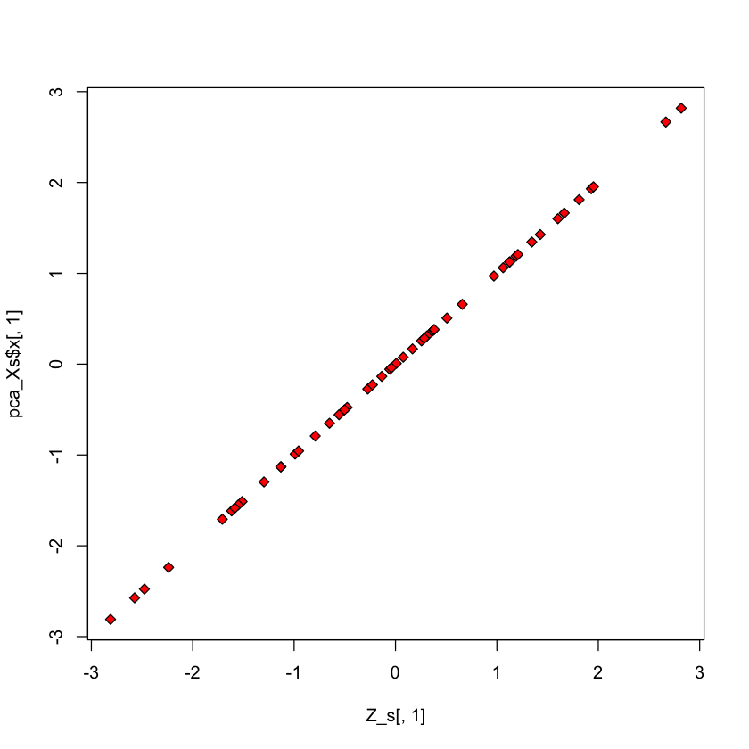
Check scores#
plot(Z_s[,1], pca_Xs$x[,1], pch=23, bg='red')
Some example applications#
USArrests data#
#| echo: true
pr.out = prcomp(USArrests, scale = TRUE)
names(pr.out)
- 'sdev'
- 'rotation'
- 'center'
- 'scale'
- 'x'
Output of prcomp#
The center and scale components correspond to the means and standard deviations of the variables that were used for scaling prior to computing SVD
#| echo: true
pr.out$center
pr.out$scale
- Murder
- 7.788
- Assault
- 170.76
- UrbanPop
- 65.54
- Rape
- 21.232
- Murder
- 4.35550976420929
- Assault
- 83.3376608400171
- UrbanPop
- 14.4747634008368
- Rape
- 9.36638453105965
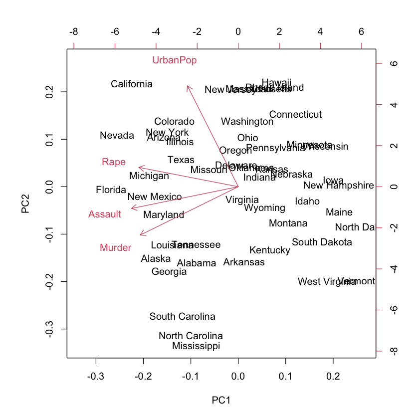
Rotation / loading#
#| echo: true
pr.out$rotation
| PC1 | PC2 | PC3 | PC4 | |
|---|---|---|---|---|
| Murder | -0.5358995 | -0.4181809 | 0.3412327 | 0.64922780 |
| Assault | -0.5831836 | -0.1879856 | 0.2681484 | -0.74340748 |
| UrbanPop | -0.2781909 | 0.8728062 | 0.3780158 | 0.13387773 |
| Rape | -0.5434321 | 0.1673186 | -0.8177779 | 0.08902432 |
Biplot#
#| echo: true

biplot(pr.out)
Variance explained#
#| echo: true
pr.out$sdev
pr.var = pr.out$sdev^2
pr.var
- 1.57487827439123
- 0.994869414817765
- 0.597129115502526
- 0.41644938195396
- 2.48024157914949
- 0.989765152539841
- 0.35656318058083
- 0.173430087729835
par(mfrow = c(1, 2))
pve = pr.var / sum(pr.var)
plot(pve, xlab = "Principal Component",
    ylab = "Proportion of Variance Explained", ylim = c(0, 1),
    type = "b")
plot(cumsum(pve), xlab = "Principal Component",
    ylab = "Cumulative Proportion of Variance Explained",
    ylim = c(0, 1), type = "b")

Congressional voting records (1984) – UCI#
#| echo: true
voting_data = read.csv('https://archive.ics.uci.edu/ml/machine-learning-databases/voting-records/house-votes-84.data', header=FALSE)
head(voting_data)
voting_X = c()
for (i in 2:7) {
voting_data[,i] = factor(voting_data[,i], c('n', '?', 'y'), ordered=TRUE)
voting_X = cbind(voting_X, as.numeric(voting_data[,i]))
}
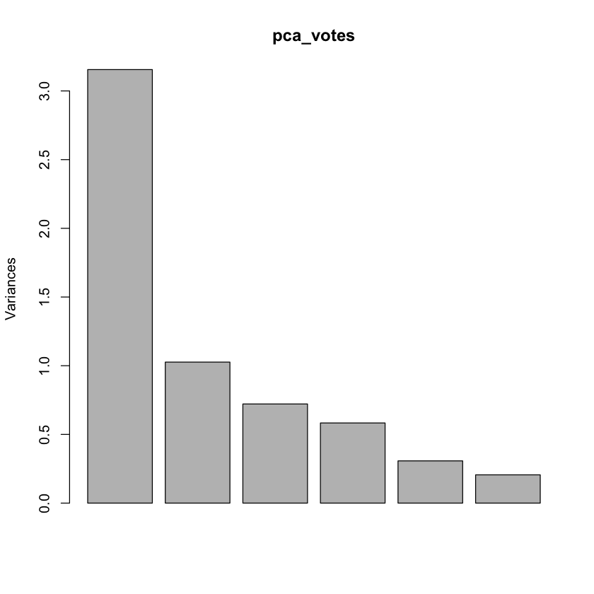
pca_votes = prcomp(voting_X, scale.=TRUE)
dem = voting_data[,1] == 'democrat'
repub = !dem
| V1 | V2 | V3 | V4 | V5 | V6 | V7 | V8 | V9 | V10 | V11 | V12 | V13 | V14 | V15 | V16 | V17 | |
|---|---|---|---|---|---|---|---|---|---|---|---|---|---|---|---|---|---|
| <chr> | <chr> | <chr> | <chr> | <chr> | <chr> | <chr> | <chr> | <chr> | <chr> | <chr> | <chr> | <chr> | <chr> | <chr> | <chr> | <chr> | |
| 1 | republican | n | y | n | y | y | y | n | n | n | y | ? | y | y | y | n | y |
| 2 | republican | n | y | n | y | y | y | n | n | n | n | n | y | y | y | n | ? |
| 3 | democrat | ? | y | y | ? | y | y | n | n | n | n | y | n | y | y | n | n |
| 4 | democrat | n | y | y | n | ? | y | n | n | n | n | y | n | y | n | n | y |
| 5 | democrat | y | y | y | n | y | y | n | n | n | n | y | ? | y | y | y | y |
| 6 | democrat | n | y | y | n | y | y | n | n | n | n | n | n | y | y | y | y |
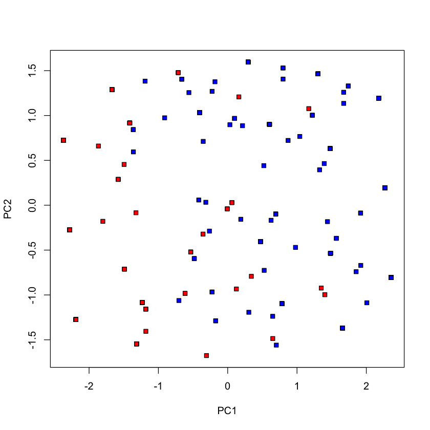
#| echo: true
plot(pca_votes$x[,1], pca_votes$x[,2], type='n', xlab='PC1', ylab='PC2')
points(pca_votes$x[dem, 1], pca_votes$x[dem, 2], pch=22, bg='blue')
points(pca_votes$x[repub, 1], pca_votes$x[repub, 2], pch=22, bg='red')
dim(voting_data)
- 435
- 17
plot(pca_votes)
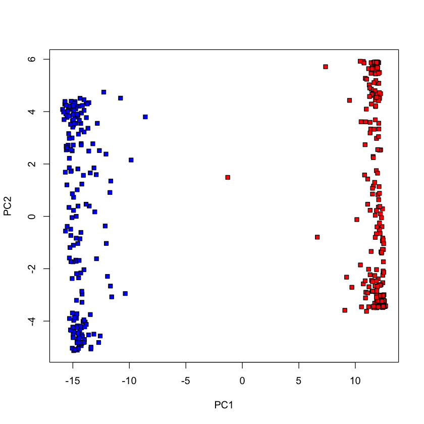
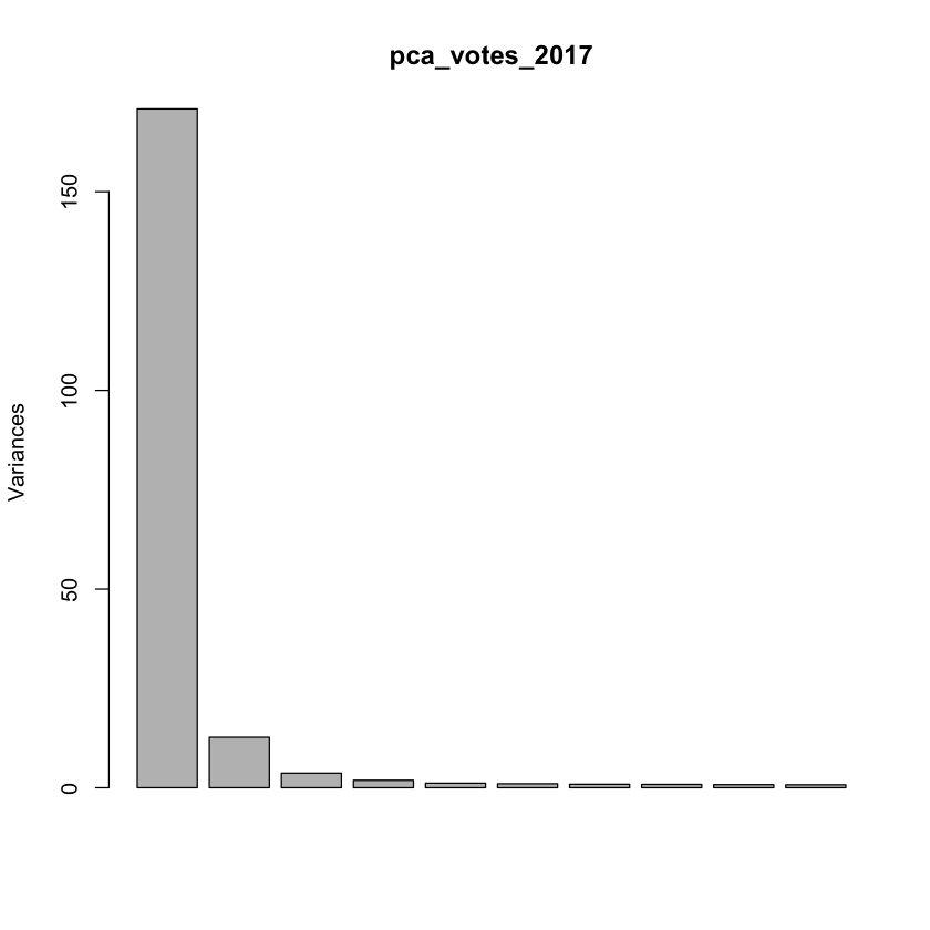
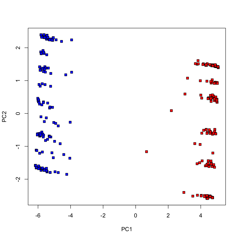
Congress of 2017#
voting_2017 = read.csv('http://stats305c.stanford.edu/data/votes2017.csv', header=TRUE)
dim(voting_2017)
dem_2017 = voting_2017$party == 'D'
repub_2017 = !dem_2017
pca_votes_2017 = prcomp(voting_2017[,-1], scale.=FALSE)
plot(pca_votes_2017$x[,1], pca_votes_2017$x[,2], type='n', xlab='PC1', ylab='PC2')
points(pca_votes_2017$x[dem_2017, 1], pca_votes_2017$x[dem_2017, 2], pch=22, bg='blue')
points(pca_votes_2017$x[repub_2017, 1], pca_votes_2017$x[repub_2017, 2], pch=22, bg='red')
- 422
- 709
plot(pca_votes_2017)
Fewer votes (randomly chosen 100 votes)#
set.seed(0)
voting_2017_fewer = voting_2017[,-1]
voting_2017_fewer = voting_2017_fewer[,sample(1:ncol(voting_2017_fewer), 100, replace=FALSE)]
pca_votes_2017_fewer = prcomp(voting_2017_fewer, scale.=FALSE)
plot(pca_votes_2017_fewer$x[,1], pca_votes_2017_fewer$x[,2], type='n', xlab='PC1', ylab='PC2')
points(pca_votes_2017_fewer$x[dem_2017, 1], pca_votes_2017_fewer$x[dem_2017, 2], pch=22, bg='blue')
points(pca_votes_2017_fewer$x[repub_2017, 1], pca_votes_2017_fewer$x[repub_2017, 2], pch=22, bg='red')
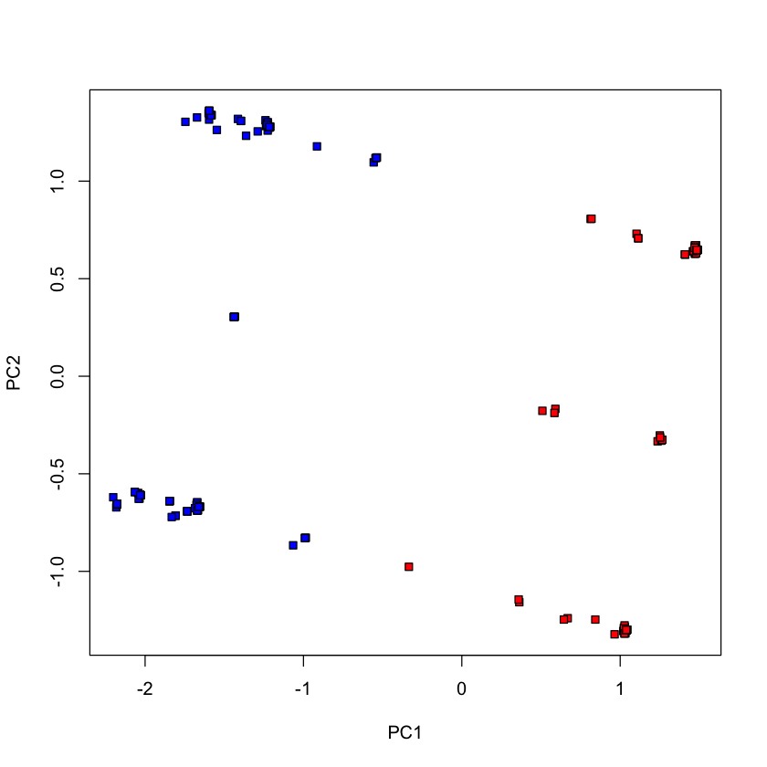
Fewer votes (randomly chosen 20 votes)#
voting_2017_fewer = voting_2017[,-1]
voting_2017_fewer = voting_2017_fewer[,sample(1:ncol(voting_2017_fewer), 20, replace=FALSE)]
pca_votes_2017_fewer = prcomp(voting_2017_fewer, scale.=FALSE)
plot(pca_votes_2017_fewer$x[,1], pca_votes_2017_fewer$x[,2], type='n', xlab='PC1', ylab='PC2')
points(pca_votes_2017_fewer$x[dem_2017, 1], pca_votes_2017_fewer$x[dem_2017, 2], pch=22, bg='blue')
points(pca_votes_2017_fewer$x[repub_2017, 1], pca_votes_2017_fewer$x[repub_2017, 2], pch=22, bg='red')
Flow cytometry data#
#| echo: true
flow = read.table('http://www.stanford.edu/class/stats305c/data/sachs.data', sep=' ', header=FALSE)
dim(flow)
plot(prcomp(flow, center=TRUE, scale.=TRUE))
- 7466
- 11
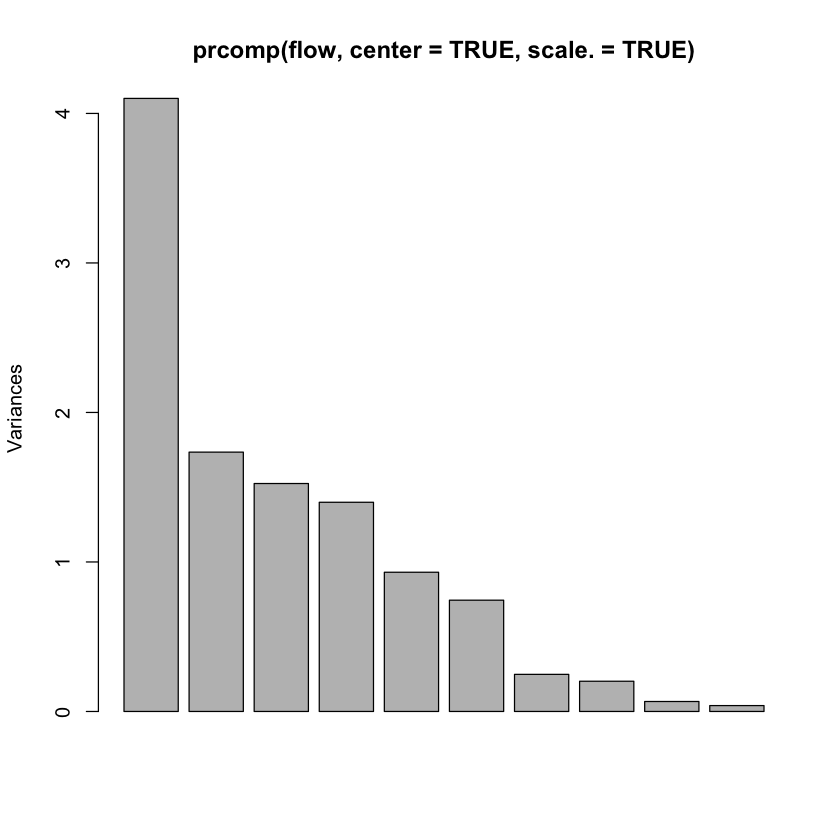
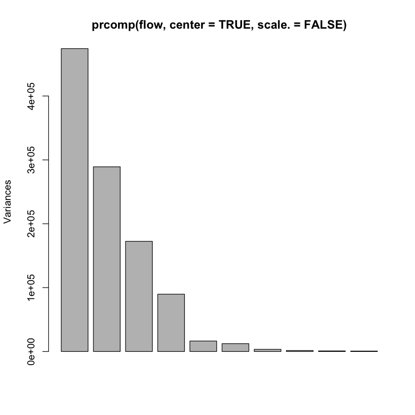
A rank 4 model?#
plot(prcomp(flow, center=TRUE, scale.=FALSE)) # rank 4?
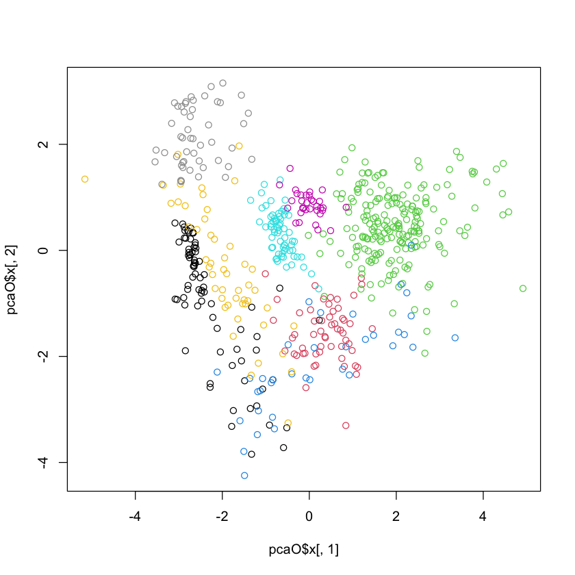
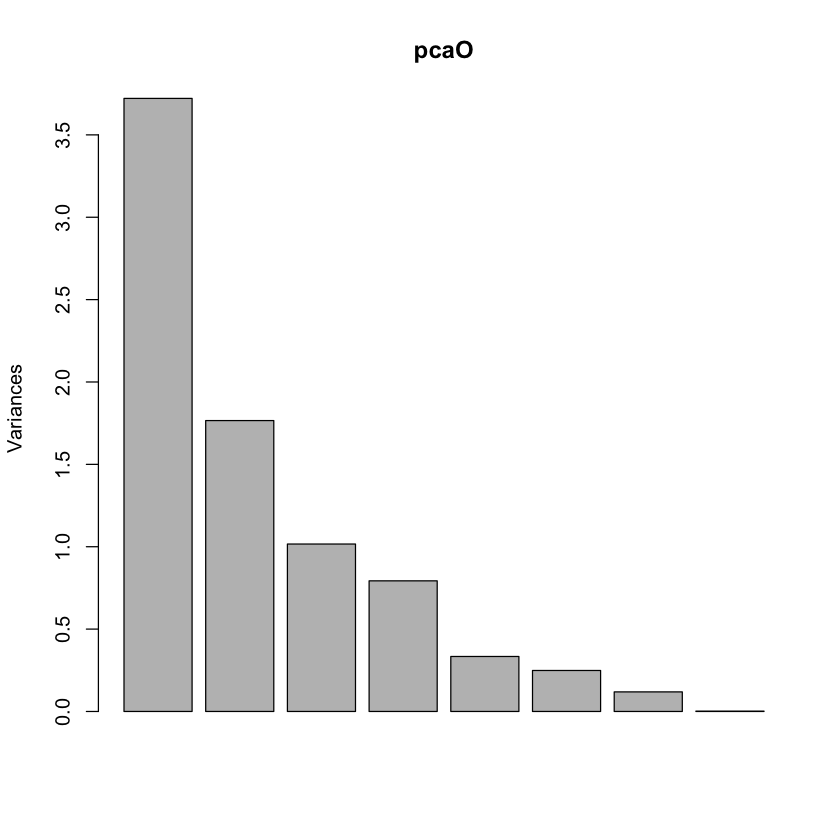
Olive oil data#
#| echo: true
library(pdfCluster)
data(oliveoil)
featO = oliveoil[,3:10]
pcaO = prcomp(featO, scale.=TRUE, center=TRUE)
plot(pcaO)
pdfCluster 1.0-4
#| echo: true
plot(pcaO$x[,1], pcaO$x[,2], col=oliveoil[,'macro.area'])
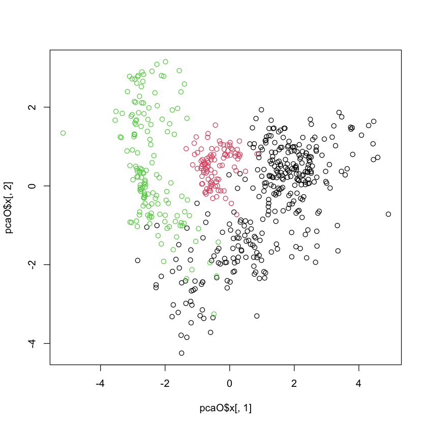
#| echo: true
plot(pcaO$x[,1], pcaO$x[,2], col=oliveoil[,'region'])