Penalized discriminants#
Download#
Penalized Discriminant Analysis#
Builds on the connection between CCA and LDA
We will follow (in some fashion):
Flexible Discriminant Analysis Hastie, Tibshirani, Buja (1993)
Penalized Discriminant Analysis Hastie, Buja, Tibshirani (1995)
Chapter 12 of ESL
References refer to optimal scoring (OS), we will not…
Takeaways#
Turns regression procedure
Y ~ Xinto a discriminant classifierY: one-hot encoding of classesX: features
Ideal for ridge-type smoothing
Outline#
All of multivariate analysis:
lm(Y ~ X)andsvd()Laplacians and smoothing
Most of the time \(Y\), \(X\) will be random vectors rather than data matrices (exceptions will hopefully be clear from context)
Smooth LDA for digits#
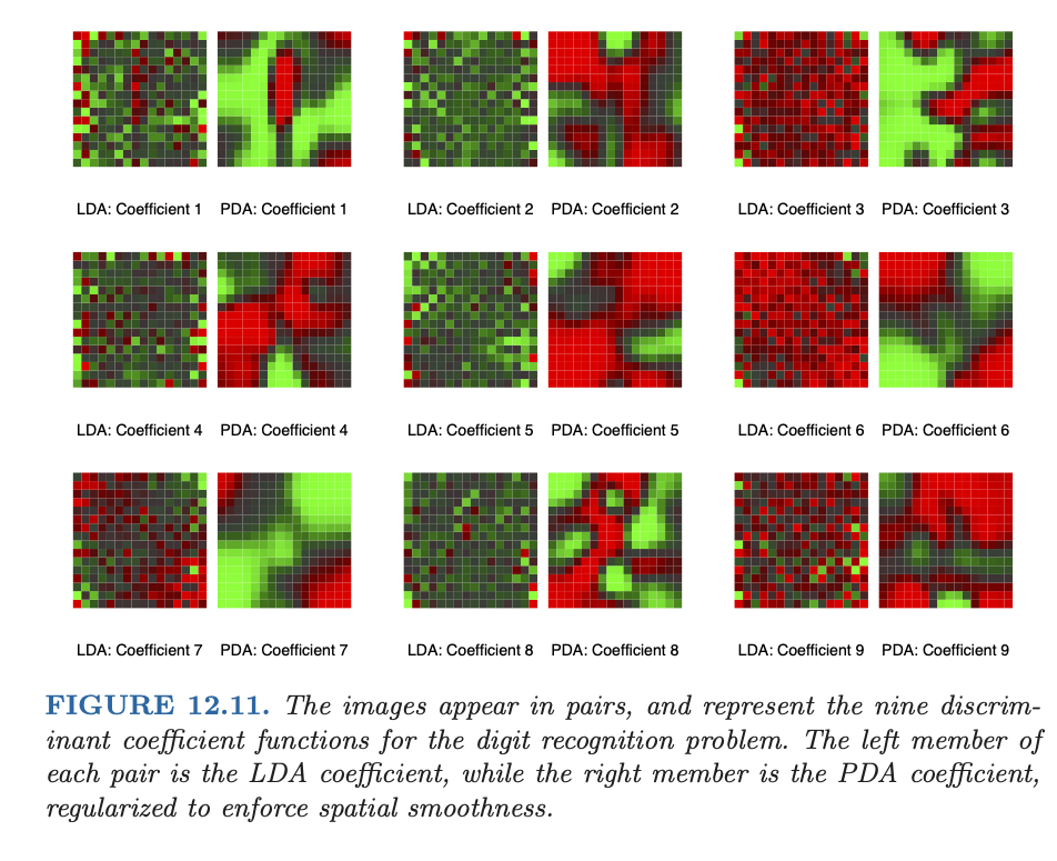
(Source: ESL)
CCA’s generalized eigenvalue problems#
In CCA, we looked at eigen-decompositions of
Setting \(A_Y'=\Sigma_{YY}^{-1/2}U_Y\) yields solutions
with
Yielded the canonical variates
Matrix form#
For non-singular \(A_X, A_Y\)
Projection version#
Let \(P_X, P_Y\) denote the correspond projections (either sample or population) of centered \(X, Y\)
Population version#
\(P_X\) projection onto \(\text{span}((X_i - \mathbb{E}[X_i]), 1 \leq i \leq p)\) in \(L^2(\mathbb{P})\)
Sample version#
With \(R_C=I-P_C=I-n^{-1}11'\), we see that
projects onto \(\text{span}((X_i - \mathbb{E}[X_i]), 1 \leq i \leq p)\) in \(L^2(\widehat{\mathbb{P}})\)
Canonical variates#
Regression in terms of canonical variates#
Straightforward to check
\(\implies\) \(X\) uses \(\Lambda Z_X\) to predict \(Z_Y\)
Given nominal OLS fits \(\hat{Y}=B'X\) (\(B=\Sigma_{XX}^{-1}\Sigma_{XY}\)) we can conclude that \(A_YB'X=A_Y\hat{Y}\) predicts \(Z_Y\).
\(\implies\) \(A_YB'X=\Lambda Z_X\)!
Reduced rank regression#
Claim:
Almost OS of Hastie et al.
Regression in original space#
By equivariance of regression
Reduced rank#
Connection to multivariate linear regression#
Consider regression
Y ~ X(burying1within \(X\))
Recall the sample quantities
Population quantities
CCA eigenvalues and multivariate regression#
The generalized eigenvalue problem we considered above is
\(\implies\) \(\Lambda^2\) are eigenvalues of \(H(H+E)^{-1}\)
Swapping \(X\) and \(Y\) shows these are the same eigenvalues for the regression
X ~ Y(with \(Q^X_T, Q^X_E, Q^X_R\))In LDA model
X ~ Yreally is multivariate linear regression…
So what? (Back to LDA)#
Two key observations (implicit / semi-explicit in ESL)#
\(\Sigma_{YY}^{-1/2}Q_R\Sigma_{YY}^{-1/2}= U_Y\Lambda^2 U_Y'\)
\(\implies\) we can find \(A_Y=\Sigma_{YY}^{-1/2}U_Y\)
Given \(A_Y\) and \(BX\) we can assume \(A_YB'X\) predicts \(A_YY=Z_Y\).
Combiined: \(\implies\) \(A_YB'X = \Lambda Z_X, \iff Z_X=\Lambda^{-1}A_YB'X = \Lambda^{-1}A_Y\hat{Y}(X)\)
Fisher’s discriminants from canonical variates#
CCA (equivalent) eigenproblems (with \(a_{i,X}'\Sigma_{XX} a_{j,X} = \delta_{ij}\))
LDA (equivalent) eigenproblems
Desiderata: find eigenvectors \(\alpha_i\) and normalize \(\alpha_{i,X}'\Sigma_{X,W}\alpha_{j,X} = \delta_{ij}\)
Equivalence of eigenproblems#
Claim#
We can take
Proof of claim#
Eigenvalue#
Aside#
\(\implies\) reduced rank regression with \(Q_T\) is equivalent to using \(Q_E\): (c.f. exercise 3.22 of ESL)
Normalization#
Sample version (almost)#
For one-hot data
Y, fitlm(Y ~ X)and formY_hat = predict(X)Compute
Compute eigendecomposition
Set \(\hat{A}_Y = (\text{SST}/n)^{-1/2} \hat{U}_Y\) and adjusted fits \(\hat{Y}\hat{A}_Y'\).
Matrix of discriminant scores are
Reduced rank LDA: just use first \(k\) of the \(\hat{V}\)’s
Why almost?#
For
Y, the matrix \(\text{SST}\) is rank-deficient as \(1'Y=1\) for one-hot data\(\implies \hat{\pi} \in \text{null(SST)}...\)
Solution#
Take \(\Theta_{K-1 \times K}\) whose column space is \(\text{row(SST)}\) with normalization
Run the above procedure on
Y @ Theta.T
This is genius!#
Algorithm#
def fit(self, X, Y):
    self.reg_estimator.fit(X, Y)
    self.A_Y, self.L = solve_eigenproblem(Y, self.reg_estimator.predict(X))
    Z = self.transform(X)
    self.centroids = class_average(Z, Y)
    return self

def transform(self, x_new)
    yhat_new = self.reg_estimator.predict(x_new)
    return (yhat_new @ self.A_Y.T / np.sqrt(L**2 * (1 - L**2))[None,:])[:,:self.rank]

def predict(self, x_new):
    V_new = self.transform(x_new)
    return np.argmin(distance(V_new, centroids), axis=1)
A pause#
Relied on (generalized) eigen decomposition of \(Y'\hat{Y}\)
This will be fine for (symmetric) linear estimators like ridge
Easy to generalize this with a basis expansion
What does it all mean?#
We motivated / derived the algorithm for
lm(Y ~ X)…For ridge, simply replace \(\Sigma_{XX}=\Sigma_{XX} + \gamma \cdot I\) above
Corresponds to regularized CCA
\(\implies\) resulting \(Z_X\)’s are regularized canonical variates as are discriminants \(V\).
Back to the digits#
Laplacian smoothing#
The application used in ESL and Hastie, Buja, Tibshirani (1995) considers features that are \(16 \times 16\) grayscale images.
Given an undirected graph \(G=(V,E)\) (like the \(16 \times 16\) lattice in 2D), define the difference operator (after orienting edges) \(D:\mathbb{R}^V \to \mathbb{R}^E\)
The Laplacian (non-negative definite version) is the map \(\Delta: \mathbb{R}^V \times \mathbb{R}^V\)
Regression problem: for digit \(d\), \(X\) the stack of images
Degrees of freedom#
For a (usually symmetric) linear smoother \(S:\mathbb{R}^n \to \mathbb{R}^n\)
Chosen to be about 40 for each digit \(d\).
Laplacian and manifold learning#
Early 2000s saw an explosion in interest in Laplacians
Given noisy \(W = \mu + \epsilon \in \mathbb{R}^V\) can smooth
Prior variance is \(\Delta^{\dagger}\) (not invertible as \(\Delta 1=0\)): \(\implies\) more weight on functions with small eigenvalues
Intuition from Laplacian on \(\mathbb{R}^k\)#
For \(f \in \mathbb{C}^2(\mathbb{R}^k)\)
Eigenfunctions#
Functions with small eigenvalues are smoother than higher eigenvalues…
Generalizations#
Take \(\alpha: [0,\infty) \to [0, \infty)\) and consider
Easy to apply given eigen decomposition of \(\Delta\)
Graph Neural Net: for graph-based features, parameterize / learn \(\alpha\)
Generators#
Taking \(\alpha(v)=v\), \(\Delta\) is (discrete-time) generator of random walk on the graph…
Taking \(\alpha(v)=e^{-tv}\), \(e^{-t\Delta}\) is the transition kernel for continuous-time random walk…
In Euclidean space \(e^{-t\Delta}\) forms the transition probabilities for Brownian motion…
Niyogi and Belkin (2001)#
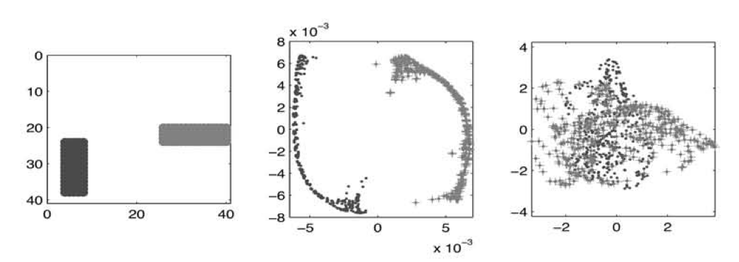
Laplacian embedding better than PCA!
Laplacian embedding#
Rough description#
Given samples \(X_i, 1 \leq i \leq n\) in some metric space \((T, d)\), construct a graph \(G_n\) with Laplacian \(\Delta_n\)
Compute low-rank eigen decomposition (of smallest eigenfunctions!)
“Embed” in \(\mathbb{R}^k\) for some user chosen rank \(k\):
At least locally, we hope (?)
A version of kernel PCA (with data-dependent kernel)
Why do we hope?#
Suppose \(T\) is a Riemannian manifold \((M,g)\) that is densely sampled by the empirical measure \(\hat{\mathbb{P}}\)
Maybe \(\hat{\mathbb{P}}\) is close to Riemannian measure \(\mu\)
We hope \(L_n\) “look like” eigenfunctions of Laplacian associated to \((M,g)\)
Why do we care about \(x \mapsto (\lambda_i^{-1/2} f_i(x))_{1 \leq i \leq k} = E_k(x)\)?
A kernel of hope#
Consider
For appropriate choices of \(\alpha\), \({\cal H}_{\alpha}\) is an RKHS! (c.f. Sobolev embedding)
Set
And…
Fact: given any covariance kernel \(K:T \times T \to \mathbb{R}\), the map \(d(x,y) = \|K_x-K_y\|_{\cal H}\) is a (pseudo-metric) on \(T\)…
\(\implies\) if \(d^2(x,y) = \|K_{\alpha}(x) - K_{\alpha}(y)\|^2_{\cal H}\) then \(E_k\) are approximate embeddings…
This assumption implies our metric was Euclidean (in some asymptotic sense). Not all metrics are Euclidean…
Related differential geometry: Spectral geometry