PCA II#
Download#
Principal components regression#
Supervised setting with response \(Y\) and design \(X\): model
where \(\alpha = \Gamma^T\beta\) and \(\text{Var}_F(X) = \Gamma \Lambda \Gamma^T\) and \(Z=X\Gamma\).
For sample version take \(\Gamma=V\) in SVD of \(R_cX\) so \(Z=\hat{Z}\)
We might hypothesize the \(\alpha[(k+1):p] = 0\), i.e. only the first \(k\) principal components of \(X\) contribute to regression…
Estimation is easy
Example of Principal Components Regression#
#| echo: true
prostate = read.table('http://www.stanford.edu/class/stats305c/data/prostate.data', header=TRUE)
M = lm(lpsa ~ . - train, data=prostate)
X = model.matrix(M)[,-1]
summary(M)
Call:
lm(formula = lpsa ~ . - train, data = prostate)

Residuals:
     Min       1Q   Median       3Q      Max
-1.76644 -0.35510 -0.00328  0.38087  1.55770

Coefficients:
             Estimate Std. Error t value Pr(>|t|)
(Intercept)  0.181561   1.320568   0.137  0.89096
lcavol       0.564341   0.087833   6.425 6.55e-09 ***
lweight      0.622020   0.200897   3.096  0.00263 **
age         -0.021248   0.011084  -1.917  0.05848 .
lbph         0.096713   0.057913   1.670  0.09848 .
svi          0.761673   0.241176   3.158  0.00218 **
lcp         -0.106051   0.089868  -1.180  0.24115
gleason      0.049228   0.155341   0.317  0.75207
pgg45        0.004458   0.004365   1.021  0.31000
---
Signif. codes:  0 ‘***’ 0.001 ‘**’ 0.01 ‘*’ 0.05 ‘.’ 0.1 ‘ ’ 1

Residual standard error: 0.6995 on 88 degrees of freedom
Multiple R-squared:  0.6634,	Adjusted R-squared:  0.6328
F-statistic: 21.68 on 8 and 88 DF,  p-value: < 2.2e-16
#| echo: true
prostate$Z = prcomp(X, center=TRUE, scale.=TRUE)$x
prcomp_reg3 = lm(lpsa ~ Z[,1:3], data=prostate)
summary(prcomp_reg3)
Call:
lm(formula = lpsa ~ Z[, 1:3], data = prostate)

Residuals:
     Min       1Q   Median       3Q      Max
-1.92094 -0.42694 -0.03113  0.52694  1.48932

Coefficients:
            Estimate Std. Error t value Pr(>|t|)
(Intercept)  2.47839    0.07661  32.352  < 2e-16 ***
Z[, 1:3]PC1  0.43188    0.04201  10.282  < 2e-16 ***
Z[, 1:3]PC2  0.07136    0.05998   1.190    0.237
Z[, 1:3]PC3  0.38651    0.07796   4.958 3.19e-06 ***
---
Signif. codes:  0 ‘***’ 0.001 ‘**’ 0.01 ‘*’ 0.05 ‘.’ 0.1 ‘ ’ 1

Residual standard error: 0.7545 on 93 degrees of freedom
Multiple R-squared:  0.5861,	Adjusted R-squared:  0.5728
F-statistic:  43.9 on 3 and 93 DF,  p-value: < 2.2e-16
#| echo: true
anova(prcomp_reg3, M)
| Res.Df | RSS | Df | Sum of Sq | F | Pr(>F) | |
|---|---|---|---|---|---|---|
| <dbl> | <dbl> | <dbl> | <dbl> | <dbl> | <dbl> | |
| 1 | 93 | 52.94137 | NA | NA | NA | NA |
| 2 | 88 | 43.05842 | 5 | 9.88295 | 4.039626 | 0.002395333 |
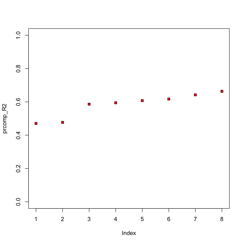
prcomp_R2 = c()
for (i in 1:8) {
    prcomp_reg = lm(lpsa ~ Z[,1:i], data=prostate)
    prcomp_R2 = c(prcomp_R2, summary(prcomp_reg)$r.squared)
}
plot(prcomp_R2, ylim=c(0,1), pch=22, bg='red')
Variations on PCA#
Matrix completion#
Source: Wikipedia
This was the task for the Netflix prize
Noisy version#
We imagine an ideal
We observe entries of \(Y\) only on \(\Omega \subset \{(i,j):1 \leq i \leq n, 1 \leq j \leq p\}\).
Goal is to estimate \(\mu\).
Natural problem to try to solve:
Needs some regularization… low-rank?
Nuclear norm#
Noiseless case#
When \(\sigma=0\) important work on the Netflix prize considered the problem
Nuclear norm: if \(\mu=UDV^T\):
Noisy case: Soft Impute#
Authors note that the data and estimate are “sparse + low-rank”
Algorithm involves repeated calls of nuclear norm proximal map (this soft-thresholds the singular values…)
When solution is low-rank the proximal map can be computed very quickly (faster than a full SVD) due to “sparse + low-rank” structure
PCA as an autoencoder#
Recall that the rank \(k\) PCA solution can be recast (with some particular choices) as
The map \(\mathbb{R}^p \ni x \mapsto Ax \in \mathbb{R}^k\) is a “low-dimensional projection” say \(P_A\).
The map \(\mathbb{R}^k \ni u \mapsto B^Tu \in \mathbb{R}^p\) is an embedding, say \(E_B\).
We could rewrite this objective as
No (strict) reason to parametrize the projection and reconstruction by linear maps…
\(\implies\) PCA is a (vanilla) version of an auto-encoder…

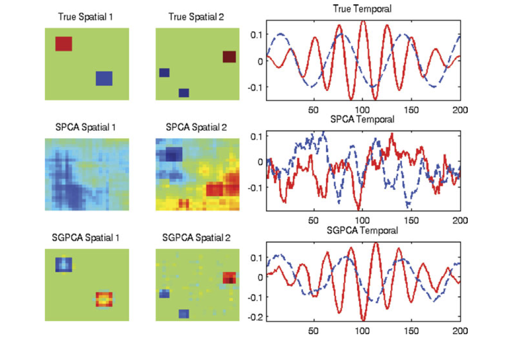
Structured PCA#
Sparse PCA#
We may want to interpret loading vectors: “what features are important for determining major modes of variation in the data?”
Why not try to make them sparse?
Rank-1 PCA has left and right singular vectors \(u, v\) that satisfy
Leading singular value is achieved value \(\hat{u}^TX\hat{v}\).
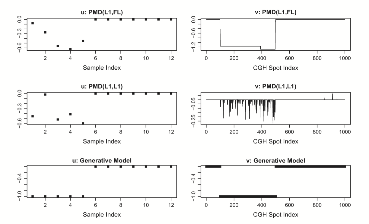
Penalized Matrix Decomposition#
Suppose we want sparsity in \(v\), the PMD proposes
Problem (phrased as minimization) is bi-convex in \((u,v)\) which induces a natural ascent algorithm: starting at \((u^{(t)}, v^{(t)})\)
Can have structure inducing penalty for \(u\) as well…
Beyond rank 1? Not as clear how to deflate as in PCA…
Missing data#
PMD can be fit with missing entries: as in matrix completion, replace \(u^TXv\) with
Iterative solution
Choice of tuning parameter#
Split \(X\) into 10 matrices removing elements at random, resulting in matrices similar to matrix completion
Run CV: fit PMD on the union of 9 out of 10, predict on missing 10th…
Similar to a scheme proposed for tuning PCA Bi-CV
CGH (copy number data)#

Fused LASSO#
They use the fused LASSO:
Solutions generically will be sparse and piecewise constant.
PMD with fused LASSO#
Non-negative matrix factorization#
We may want other structure in factors
If \(X_{ij} > 0\) (e.g. count data) we may consider (constraints considered elementwise)
Natural model for NNMF?#
Suppose
Under independence model
Corresponds to sampling a Poisson number of individuals from a population with \(R\) independent of \(C\).
Suppose there is a mixture of \(k\) independence models
Such \(\lambda\) matrix has an NNMF of rank \(k\), though likelihood would not be Frobenius norm…
Structured covariance#
We looked at PCA solely with Frobenius norm, i.e. the rank \(k\) PCA is equivalent to
What if there were structure across rows, i.e. \(X[,i] \sim N(0, \Sigma_R)\)?
Reasonable to whiten first and consider
Could have structure in the columns as well, why not whiten there as well?
Replaces Frobenius norm with a norm
Frobenius is the special case \(\Sigma_C, \Sigma_R = I_p, I_n\).
Example#