Multivariate regression#
Download#
Multiple linear regression#

Response matrix: \(Y \in \mathbb{R}^{n \times q}\)
Design matrix: \(X \in \mathbb{R}^{n \times p}\)
MKB swaps \(p\) and \(q\). Here \(p\) always refers to features.
Model#
MKB uses \(U\) instead of \(\epsilon\).
Geometry of OLS still applies#
Soils example#
library(car)
data(Soils)
str(Soils)
Loading required package: carData
'data.frame':	48 obs. of  14 variables:
 $ Group  : Factor w/ 12 levels "1","2","3","4",..: 1 1 1 1 2 2 2 2 3 3 ...
 $ Contour: Factor w/ 3 levels "Depression","Slope",..: 3 3 3 3 3 3 3 3 3 3 ...
 $ Depth  : Factor w/ 4 levels "0-10","10-30",..: 1 1 1 1 2 2 2 2 3 3 ...
 $ Gp     : Factor w/ 12 levels "D0","D1","D3",..: 9 9 9 9 10 10 10 10 11 11 ...
 $ Block  : Factor w/ 4 levels "1","2","3","4": 1 2 3 4 1 2 3 4 1 2 ...
 $ pH     : num  5.4 5.65 5.14 5.14 5.14 5.1 4.7 4.46 4.37 4.39 ...
 $ N      : num  0.188 0.165 0.26 0.169 0.164 0.094 0.1 0.112 0.112 0.058 ...
 $ Dens   : num  0.92 1.04 0.95 1.1 1.12 1.22 1.52 1.47 1.07 1.54 ...
 $ P      : int  215 208 300 248 174 129 117 170 121 115 ...
 $ Ca     : num  16.4 12.2 13 11.9 14.2 ...
 $ Mg     : num  7.65 5.15 5.68 7.88 8.12 ...
 $ K      : num  0.72 0.71 0.68 1.09 0.7 0.81 0.39 0.7 0.74 0.77 ...
 $ Na     : num  1.14 0.94 0.6 1.01 2.17 2.67 3.32 3.76 5.74 5.85 ...
 $ Conduc : num  1.09 1.35 1.41 1.64 1.85 3.18 4.16 5.14 5.73 6.45 ...
Estimation of \(B\)#
Negative log-likelihood#
As in one-sample problem
Score equation (assuming \(\Sigma >0\))
Estimation of \(\Sigma\)#
For \(\hat{\Sigma}_{MLE}>0\) we need \(\text{rank}(I-P_F) \geq q\) which is generic if \(n-p \geq q\).
Unbiased estimate#
Minimized (negative) log-likelihood#
As in one-sample problem we see
Criterion for use e.g. in AIC, BIC…
LRT (up to multiplicative factor)#
Distribution results#
Fairly easy to check:
\(\hat{B} \sim N(B, (X^TX)^{-1} \otimes \Sigma)\)
\((n-p) \hat{\Sigma} \sim \text{Wishart}(n-p, \Sigma)\)
\(\hat{B}\) independent of \(\hat{\Sigma}\)
Sums of squares matrices#
Set \(I-P_C=I-\frac{1}{n}11^T\).
Just like
lmbut matrices…
Analogy of \(F\)-test in summary.lm#
Typically first column of \(X\) is \(1\).
Usual \(F\) test is of
Natural matrix to consider
Likelihood ratio test statistic#
Test statistic: Wilks’ Lambda (LRT/n), Roy’s maximum root: largest eigenvalue, etc.
Section 6.5.4. MKB use \((H+E)^{-1}E\) as analog of \(1-R^2\): a Beta matrix under \(H_0\)
Inference#
General linear hypothesis#
Special case#
To test hypotheses of the form
Key quantities are sums of squares matrices
with
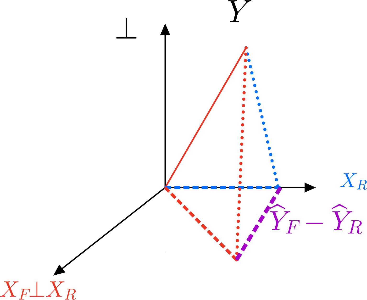
Where does \(P_F-P_R\) come from?#
Type III MANOVA#
#| echo: true
soils.full = lm(cbind(pH, N, Dens, P, Ca, Mg, K, Na, Conduc) ~
                Block + Contour * Depth,
               data=Soils)
Manova(soils.full, test.statistic="Wilks", type=3)
Type III MANOVA Tests: Wilks test statistic
              Df test stat approx F num Df  den Df    Pr(>F)
(Intercept)    1  0.006336   435.63      9  25.000 < 2.2e-16 ***
Block          3  0.079430     3.77     27  73.655 3.347e-06 ***
Contour        2  0.159872     4.17     18  50.000 3.246e-05 ***
Depth          3  0.028896     6.45     27  73.655 9.554e-11 ***
Contour:Depth  6  0.216611     0.86     54 132.070    0.7392
---
Signif. codes:  0 ‘***’ 0.001 ‘**’ 0.01 ‘*’ 0.05 ‘.’ 0.1 ‘ ’ 1
Sanity check for Block#
## Response matrix
Y = with(Soils, cbind(pH, N, Dens, P, Ca, Mg, K, Na, Conduc))

## Projection for full model
X_F = model.matrix(soils.full)
P_F = X_F %*% solve(t(X_F) %*% X_F) %*% t(X_F)

## Projection for reduced model
soils.red = lm(cbind(pH, N, Dens, P, Ca, Mg, K, Na, Conduc) ~ Contour * Depth,
               data=Soils)
X_R = model.matrix(soils.red)
P_R = X_R %*% solve(t(X_R) %*% X_R) %*% t(X_R)
Compute the LRT#
E = t(Y) %*% (diag(rep(1, nrow(Y))) - P_F) %*% Y
H = t(Y) %*% (P_F - P_R) %*% Y
wilks = det(E %*% solve(E + H))
c(wilks=wilks)
Manova(soils.full, test.statistic="Wilks", type=3)
Type III MANOVA Tests: Wilks test statistic
              Df test stat approx F num Df  den Df    Pr(>F)
(Intercept)    1  0.006336   435.63      9  25.000 < 2.2e-16 ***
Block          3  0.079430     3.77     27  73.655 3.347e-06 ***
Contour        2  0.159872     4.17     18  50.000 3.246e-05 ***
Depth          3  0.028896     6.45     27  73.655 9.554e-11 ***
Contour:Depth  6  0.216611     0.86     54 132.070    0.7392
---
Signif. codes:  0 ‘***’ 0.001 ‘**’ 0.01 ‘*’ 0.05 ‘.’ 0.1 ‘ ’ 1
Types of Sums of Squares#
Here is a good reference
For \(q=1\),
Rreturns Type I sums of squares. Arguably, Type II or III is more natural.When no interactions present, Type II will agree with Type III, otherwise can differ: see
DepthandContourbelow.When designs are balanced, Type I can agree with Type II.
# Look at rows for `Depth`
Manova(soils.full, test.statistic="Wilks", type=3) # compare to type=2
Type III MANOVA Tests: Wilks test statistic
              Df test stat approx F num Df  den Df    Pr(>F)
(Intercept)    1  0.006336   435.63      9  25.000 < 2.2e-16 ***
Block          3  0.079430     3.77     27  73.655 3.347e-06 ***
Contour        2  0.159872     4.17     18  50.000 3.246e-05 ***
Depth          3  0.028896     6.45     27  73.655 9.554e-11 ***
Contour:Depth  6  0.216611     0.86     54 132.070    0.7392
---
Signif. codes:  0 ‘***’ 0.001 ‘**’ 0.01 ‘*’ 0.05 ‘.’ 0.1 ‘ ’ 1
Type I vs. Type 2 & 3#
X = rnorm(50)
W = rnorm(50)
Z = matrix(rnorm(100), 50, 2)
anova(lm(Z ~ X + W))
Manova(lm(Z ~ X + W), type=2)
Manova(lm(Z ~ X + W), type=3)
| Df | Pillai | approx F | num Df | den Df | Pr(>F) | |
|---|---|---|---|---|---|---|
| <int> | <dbl> | <dbl> | <dbl> | <dbl> | <dbl> | |
| (Intercept) | 1 | 0.131648226 | 3.486961 | 2 | 46 | 0.038904605 |
| X | 1 | 0.185791947 | 5.248308 | 2 | 46 | 0.008849405 |
| W | 1 | 0.008329814 | 0.193195 | 2 | 46 | 0.824986612 |
| Residuals | 47 | NA | NA | NA | NA | NA |
Type II MANOVA Tests: Pillai test statistic
  Df test stat approx F num Df den Df   Pr(>F)
X  1   0.18490   5.2173      2     46 0.009076 **
W  1   0.00833   0.1932      2     46 0.824987
---
Signif. codes:  0 ‘***’ 0.001 ‘**’ 0.01 ‘*’ 0.05 ‘.’ 0.1 ‘ ’ 1
Type III MANOVA Tests: Pillai test statistic
            Df test stat approx F num Df den Df   Pr(>F)
(Intercept)  1  0.086252   2.1711      2     46 0.125606
X            1  0.184897   5.2173      2     46 0.009076 **
W            1  0.008330   0.1932      2     46 0.824987
---
Signif. codes:  0 ‘***’ 0.001 ‘**’ 0.01 ‘*’ 0.05 ‘.’ 0.1 ‘ ’ 1
Other test statistics: Roy’s maximum root#
Based on the union-intersection principle using the family
For each \(a\) we can test \(H_{0,a}\) with an \(F\)-test
Ignoring factor \((n-p)/k\) we then maximize over \(a\)
Computing Roy’s maximum root#
#| echo: true
eigvals = as.numeric(eigen(H %*% solve(E))$values)
roy = max(eigvals); roy
Manova(soils.full, test.statistic="Roy", type=3)
Warning message:
“imaginary parts discarded in coercion”
Type III MANOVA Tests: Roy test statistic
              Df test stat approx F num Df den Df    Pr(>F)
(Intercept)    1   156.827   435.63      9     25 < 2.2e-16 ***
Block          3     2.219     6.66      9     27 5.625e-05 ***
Contour        2     2.705     7.82      9     26 1.739e-05 ***
Depth          3    14.251    42.75      9     27 1.126e-13 ***
Contour:Depth  6     0.902     3.01      9     30   0.01113 *
---
Signif. codes:  0 ‘***’ 0.001 ‘**’ 0.01 ‘*’ 0.05 ‘.’ 0.1 ‘ ’ 1
Hotelling-Lawley trace#
Test statistic: \(\text{Tr}(HE^{-1})\).
lawley = sum(eigvals)
c(lawley=lawley)
Manova(soils.full, test.statistic="Hotelling-Lawley", type=3)
Type III MANOVA Tests: Hotelling-Lawley test statistic
              Df test stat approx F num Df den Df    Pr(>F)
(Intercept)    1   156.827   435.63      9     25 < 2.2e-16 ***
Block          3     4.183     3.67     27     71 6.188e-06 ***
Contour        2     3.394     4.52     18     48 1.443e-05 ***
Depth          3    15.480    13.57     27     71 < 2.2e-16 ***
Contour:Depth  6     1.954     0.84     54    140    0.7585
---
Signif. codes:  0 ‘***’ 0.001 ‘**’ 0.01 ‘*’ 0.05 ‘.’ 0.1 ‘ ’ 1
Pillai-Bartlett trace#
Test statistic: \(\text{Tr}((I + HE^{-1})^{-1})) = \text{Tr}(E(E+H)^{-1}).\)
pillai = sum(eigvals / (1 + eigvals))
c(pillai=pillai)
Manova(soils.full, test.statistic="Pillai", type=3)
Type III MANOVA Tests: Pillai test statistic
              Df test stat approx F num Df den Df    Pr(>F)
(Intercept)    1   0.99366   435.63      9     25 < 2.2e-16 ***
Block          3   1.67579     3.80     27     81 1.777e-06 ***
Contour        2   1.13773     3.81     18     52 8.025e-05 ***
Depth          3   1.51137     3.05     27     81 6.020e-05 ***
Contour:Depth  6   1.23510     0.86     54    180    0.7311
---
Signif. codes:  0 ‘***’ 0.001 ‘**’ 0.01 ‘*’ 0.05 ‘.’ 0.1 ‘ ’ 1
Finding Sum of Squares from Manova#
M = Manova(soils.full)
sqrt(sum((M$SSPE - E)^2))
sqrt(sum((M$SSP$Block - H)^2))
Tests about different responses#
We might sometimes be interested in testing a hypothesis of the form
For example, the hypothesis that all \(q\) coefficient vectors are identical
Reduced response#
In this case, we use response vector \(\widetilde{Y}=YM\) and the model
Our hypothesis here can be expressed as \(\widetilde{B}=0\).
Hence, the relevant sums of squares are
q = ncol(Y)
M = (diag(rep(1, q)) - matrix(1, q, q) / q)[,1:(q-1)]
E_new = t(M) %*% E %*% M
H_new = t(M) %*% (t(Y) %*% Y - E) %*% M
roy = max(as.numeric(eigen(H_new %*% solve(E_new))$values)); roy
Combining both types of tests#
To test \(H_0: CBM=0\), we use
Affine shifts#
Finally, suppose \(h \neq 0\)
For this, take any fixed \(B_0 \in H_0\) such that \(CB_0M=h\) and set
with \(\Delta=B-B_0\).
Our null is now \(H_0:C\Delta M=0\) and we can use