Structured

Download

• HTML

• Rmd

• PDF

---

• Fixing \(\Sigma\), solve for \(\gamma\)

\[ \widehat{\gamma}(\Sigma, X, Y) = (X^TX)^{-1}X^T\frac{Y \Sigma^{-1} 1}{1^T\Sigma^{-1}1} \]

• Solving for optimal \(\Sigma\) seems messy, could just plug in unbiased estimate

\[ \widehat{\Sigma} = Y^T(I-P_F)Y / (n-p). \]

---

TRUE

TRUE

Reduced rank regression: rank 1

• The null \(H_0:B(I - \frac{1}{q}11^T)=0\) says that \(B=\gamma 1^T\), i.e. the \(q\) different regressions share parameters \(\gamma\).

• This imposes some structure on \(B\). In this case \(B\) is rank 1 (and we have fixed its row space).

• A natural generalization is to remove constraint that row space is \(1\):

\[ B = UV^T, \qquad U \in \mathbb{R}^p, V \in \mathbb{R}^q \]

---

Model

• If we knew \(V\) $\( YV \sim N(XUV^TV, I \otimes V^T\Sigma V) = N((V^TV) \cdot XU, V^T\Sigma V \cdot I) \)$

• Design matrix has one column!

• Regression with a univariate response.

• This model says that \(Y|X\)’s variation is driven by \(XU\) though in possibly different directions determined by columns of \(V\).

---

• Fitting this model for given \(\Sigma\) we need to solve

\[ \text{min}_{U,V} - \text{Tr}(\Sigma^{-1}Y^TXUV^T) + \frac{1}{2} \text{Tr}(\Sigma^{-1}(XUV^T)^TXUV^T) \]

• Differentiate wrt \(V\) for fixed \(U\) yields score equation

\[ \Sigma^{-1}Y^TXU = \Sigma^{-1}\widehat{V}(XU)^T(XU) \implies \widehat{V}(X,Y,U) = Y^T(XU)((XU)^TXU)^{-1} \]

---

• Substituting \(\widehat{V}\) yields the problem

\[ \text{minimize}_U -\frac{1}{2} \text{Tr}\left(\Sigma^{-1}Y^TXU((XU)^TXU)^{-1}(XU)^TY\right) \]

• Many minimizers here, let’s pick one…

• Let \(\widehat{W}\) be the leading unit eigenvector of

\[ (X^TX)^{-1/2}X^TY\Sigma^{-1}Y^TX (X^TX)^{-1/2} \]

and set \(\widehat{U}=(X^TX)^{-1/2}\widehat{W}\), noting that \((X\widehat{U})^TX\widehat{U} = 1\).

• Can also plugin \(\widehat{\Sigma}=Y^T(I-P_F)Y / (n-p)\).

---

• Plugging into expression for \(V\) yields

\[ \widehat{V} = Y^TX(X^TX)^{-1/2}\widehat{W} \]

and

\[\begin{split} \begin{aligned} \widehat{U} \widehat{V}^T &= (X^TX)^{-1/2} \widehat{W} \widehat{W}^T (X^TX)^{-1/2} Y^TX \\ &= (X^TX)^{-1/2} \widehat{W} \widehat{W}^T (X^TX)^{1/2} \widehat{B} \\ \end{aligned} \end{split}\]

with \(\widehat{B}=(X^TX)^{-1}X^TY\) the unrestricted MLE.

---

• An equivalent expression

\[ \widehat{U}\widehat{V}^T = \widehat{B} \Sigma^{-1/2} \widehat{Z} \widehat{Z}^T \Sigma^{1/2} \]

where \(\widehat{Z}\) is the leading unit eigenvector of

\[ \Sigma^{-1/2}Y^TX (X^TX)^{-1}X^TY \Sigma^{-1/2} \]

---

Relation to CCA

• Common to choose \(\widehat{U}\) so that \(X\widehat{U}\) has standard deviation 1. Similarly, \(Y\widehat{V}\) is another \(n\)-vector that can be scaled to have standard deviation 1.

• In fact, any pair \(U, V\) determine two such \(n\)-vectors. We might look at

\[ \widehat{Cor}(XU, YV) = \frac{U^TX^T\widehat{\Sigma}_{XY} YV}{\left(((XU)^T\widehat{\Sigma}_{XX}XU) ((YV)^T\widehat{\Sigma}_{YY}YV)\right)^{1/2}} \]

• The maximizing \((U,V)\) are the \((\widehat{U}, \widehat{V})\) we derived above up to a scaling by the maximized correlation.

• We will revisit this when we talk about canonical correlations (Chapter 10 of MKB)

---

General case: rank \(k\)

• Let us now take \(U \in \mathbb{R}^{p \times k}, V \in \mathbb{R}^{q \times k}\) with \(k < \text{min}(n,p)\).

• Model has \(O(k(q+p))\) parameters, can be much smaller than \(qp\) if, say, \(p\) is large and \(q\) is moderate.

• Given \(U\), the optimal \(V\) is the same

\[ \widehat{V}(X,Y,U) = Y^T(XU)((XU)^TXU)^{-1} \]

---

• To find \(\widehat{U}\) we must solve $\( \text{minimize}_{U \in \mathbb{R}^{p \times k}} -\frac{1}{2} \text{Tr}\left(\Sigma^{-1}Y^TXU((XU)^TXU)^{-1}(XU)^TY\right) \)$

• Note that objective is unchanged if we replace \(U\) with \(UA\) for non-singular \(A_{k \times k}\).

• We can choose \(U\) such that \(U^T(X^TX)U=I_{k \times k}\)…

---

A very useful fact

• Suppose \(\mathbb{R}^{m \times m} \ni M=M^T \geq 0\). Consider

\[ \text{maximize}_{U \in \mathbb{R}^{m \times k}: U^TU=I_{k \times k}} \text{Tr}(MUU^T) \]

• Matrix \(M\) has an eigendecomposition:

\[ M = \sum_{i=1}^m \lambda_i V_i V_i^T \]

• If \(\lambda(M)\) has no ties at \(\lambda_k(M)\), then

\[ \hat{U} = \begin{pmatrix} V_1 & \dots & V_k \end{pmatrix} \]

• With ties in \(\lambda_i(M)\) eigendecomposition is not unique. Minimizers still formed by taking \(k\) eigenvectors corresponding to top \(k\) eigenvalues.

---

Proof:

• Von Neumann trace inequality for (symmetric) matrices \(A,B\)

\[ |\text{Tr}(AB)| \leq \sum_i |\lambda_i(A)| |\lambda_i(B)| \]

• When \(B=UU^T\) is a rank \(k\) projection and \(A \geq 0\)

\[ \text{Tr}(AB) \leq \sum_{i=1}^k \lambda_i(A) \]

• Our proposal achieves this value…

• General version of inequality with \(\sigma_i(A)\) the singular values:

\[ |\text{Tr}(AB)| \leq \sum_i \sigma_i(A) \sigma_i(B) \]

---

Finishing reduced rank

• Let \(\widehat{W}\) be such that \(\widehat{W}\widehat{W}^T\) is the (orthogonal) projection onto the rank top \(k\) eigenvectors of \((X^TX)^{-1/2}X^TY \Sigma^{-1} Y^TX (X^TX)^{-1/2}\) and set \(\widehat{U}=(X^TX)^{-1/2}\widehat{W}\).

• Answer is identical to rank 1 case, though the matrices \(\widehat{Z}, \widehat{W}\) have more than one column now.

• Common to plug in \(\widehat{\Sigma}=Y^T(I-1/n 11^T)Y/(n-1)\), though answer is the same with \(\widehat{\Sigma}=Y^T(I-P_F)Y/(n-p)\) (Exercise 3.22 in ESL).

---

Starting point

• This follows rrr vignette here

#| echo: true
library(rrr)
data(tobacco)
str(tobacco)

Attaching package: ‘rrr’

The following object is masked from ‘package:stats’:

    residuals

'data.frame':	25 obs. of  9 variables:
 $ Y1.BurnRate         : num  1.55 1.63 1.66 1.52 1.7 1.68 1.78 1.57 1.6 1.52 ...
 $ Y2.PercentSugar     : num  20.1 12.6 18.6 18.6 14 ...
 $ Y3.PercentNicotine  : num  1.38 2.64 1.56 2.22 2.85 1.24 2.86 2.18 1.65 3.28 ...
 $ X1.PercentNitrogen  : num  2.02 2.62 2.08 2.2 2.38 2.03 2.87 1.88 1.93 2.57 ...
 $ X2.PercentChlorine  : num  2.9 2.78 2.68 3.17 2.52 2.56 2.67 2.58 2.26 1.74 ...
 $ X3.PercentPotassium : num  2.17 1.72 2.4 2.06 2.18 2.57 2.64 2.22 2.15 1.64 ...
 $ X4.PercentPhosphorus: num  0.51 0.5 0.43 0.52 0.42 0.44 0.5 0.49 0.56 0.51 ...
 $ X5.PercentCalcium   : num  3.47 4.57 3.52 3.69 4.01 2.79 3.92 3.58 3.57 4.38 ...
 $ X6.PercentMagnesium : num  0.91 1.25 0.82 0.97 1.12 0.82 1.06 1.01 0.92 1.22 ...

---

Extract \(X\) and \(Y\)

#| echo: true
library(dplyr)
tobacco <- as_tibble(tobacco)
tobacco_x <- tobacco %>%
    select(starts_with("X"))

tobacco_y <- tobacco %>% 
    select(starts_with("Y"))

Attaching package: ‘dplyr’

The following objects are masked from ‘package:stats’:

    filter, lag

The following objects are masked from ‘package:base’:

    intersect, setdiff, setequal, union

---

#| echo: true
Y = as.matrix(tobacco_y)
X = as.matrix(tobacco_x)
lm(Y ~ X)

Call:
lm(formula = Y ~ X)

Coefficients:
                       Y1.BurnRate  Y2.PercentSugar  Y3.PercentNicotine
(Intercept)             1.41114     13.63291         -1.56482          
XX1.PercentNitrogen     0.06197     -4.31867          0.55216          
XX2.PercentChlorine    -0.16013      1.32629         -0.27856          
XX3.PercentPotassium    0.29212      1.58995          0.21759          
XX4.PercentPhosphorus  -0.65798     13.95265         -0.72311          
XX5.PercentCalcium      0.17303      0.55259          0.32309          
XX6.PercentMagnesium   -0.42835     -3.50211          2.00486          

---

#| echo: true
rrr(X, Y, type='identity', rank=2)

$mean

A matrix: 3 × 1 of type dbl

3.4740985

13.9605303

-0.5117545

$A

A matrix: 3 × 2 of type dbl

0.03107787	-0.4704307
-0.97005030	0.1984637
0.24090782	0.8598297

$B

A matrix: 2 × 6 of type dbl

X1.PercentNitrogen	X2.PercentChlorine	X3.PercentPotassium	X4.PercentPhosphorus	X5.PercentCalcium	X6.PercentMagnesium
4.3242696	-1.35864835	-1.4808316	-13.729424	-0.4528289	3.866896
-0.4114869	0.09903401	0.3652138	2.456879	0.3060762	1.230305

$C

A matrix: 3 × 6 of type dbl

X1.PercentNitrogen	X2.PercentChlorine	X3.PercentPotassium	X4.PercentPhosphorus	X5.PercentCalcium	X6.PercentMagnesium
0.3279651	-0.08881253	-0.21782885	-1.582473	-0.1580606	-0.4585985
-4.2764242	1.33761189	1.50896282	13.805833	0.5000118	-3.5069123
0.6879417	-0.24215663	-0.04272224	-1.195028	0.1540834	1.9894186

$eigen_values

1. 3.2820997448457
2. 0.0378297755314835
3. 0.0101599583310807

---

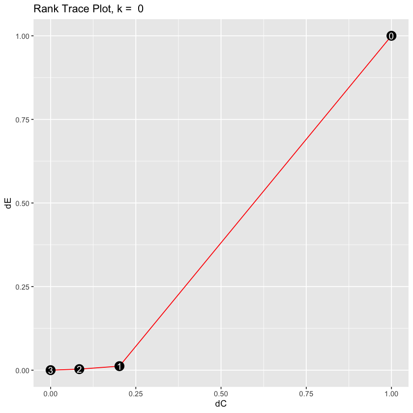
#| echo: true
rank_trace(X, Y, type='identity')

Warning message:
“`data_frame()` was deprecated in tibble 1.1.0.
ℹ Please use `tibble()` instead.
ℹ The deprecated feature was likely used in the rrr package.
  Please report the issue to the authors.”

Warning message:
“`as_data_frame()` was deprecated in tibble 2.0.0.
ℹ Please use `as_tibble()` (with slightly different semantics) to convert to a tibble, or `as.data.frame()` to convert
  to a data frame.
ℹ The deprecated feature was likely used in the rrr package.
  Please report the issue to the authors.”

Warning message:
“The `x` argument of `as_tibble.matrix()` must have unique column names if `.name_repair` is omitted as of tibble
2.0.0.
ℹ Using compatibility `.name_repair`.
ℹ The deprecated feature was likely used in the tibble package.
  Please report the issue at <https://github.com/tidyverse/tibble/issues>.”

Sparsity

LASSO?

• Of course, there are other types of structure…

• Usually \(X\) will be centered and standardized to make features comparable

\[ \text{minimize}_{B, \Sigma} \frac{n}{2} \log \left|2 \pi \Sigma \right| + \frac{1}{2} \text{Tr}(\Sigma^{-1}(Y-XB)^T(Y-XB)) + \lambda \sum_{i,j} |B_{i,j}| \]

---

• Often \(\Sigma=I\) is used: decouples likelihood into \(q\) terms

\[\begin{split} \begin{aligned} \frac{1}{2}\text{Tr}((Y-XB)^T(Y-XB)) &= \frac{1}{2}\|Y-XB\|^2_F \\ &= \frac{1}{2}\sum_{j=1}^q \|Y[,j] - XB[,j]\|^2_2 \end{aligned} \end{split}\]

• Sparsity is not shared in any sense: \(q\) separate LASSO problems $\( \text{minimize}_{B[,j], 1 \leq j \leq q} \sum_{j=1}^q \left[\frac{1}{2} \|Y[,j]-XB[,j]\|^2_2 + \lambda \|B[,j]\|_1 \right] \)$

• Some methods don’t require plugging in \(\Sigma\)

---

Group sparsity

• The blockwise group-LASSO could be used

\[ \text{minimize}_{B} \frac{1}{2} \|Y-XB\|^2_F + \lambda \sum_{i=1}^p w_i \|B[i,]\|_2 \]

• Yields solutions that zero out entire rows of \(B\) – drops some features!

• Reference: Obozinski et al.

• Sometimes \(\|\cdot\|_{\infty}\) is used.

---

Group LASSO

• Suppose \(\{1, \dots, p\}\) is partitioned as \(\{g_1, \dots, g_k\}\) (i.e. disjoint groups).

• Generically, for large values of \(\lambda\) if we solve a (convex) problem

\[ \text{minimize}_{\beta} \ell(\beta) + \lambda \sum_{j=1}^k w_j \|\beta[g_j]\|_2 \]

we will see several \(\widehat{\beta}[g_j]\) = 0. Why?

• In the multivariate regression case, grouping the rows of \(B\) together gives us solutions where several rows are exactly 0.

---

Why do we get exact zeros?

• Properties of a penalty \({\cal P}\) can be determined from its proximal map

\[ \pi_{\cal P}(y) = \text{argmin}_z \frac{1}{2} \|y-z\|^2_2 + {\cal P}(z) \]

• Let’s consider one group:

\[ \text{argmin}_z \frac{1}{2} \|y-z\|^2_2 + \lambda \|z\|_2 \]

---

• Differentiating yields equation (where differentiable)

\[ z-y + \lambda z / \|z\|_2 = 0 \]

• Clearly if there is a solution \(\widehat{z}(y) = c \cdot y\) and it is enough to solve

\[ \text{argmin}_c \frac{1}{2} \|y-cy\|^2_2 + \lambda |c| \|y\|_2 \]

• Optimal \(c\) is \(\max(1 - \lambda / \|y\|_2, 0)\):

\[ \widehat{z}(y) = y \cdot \max(1 - \lambda / \|y\|_2, 0) \]

• Norm of solution \(\max(\|y\|_2 - \lambda, 0)\): soft-thresholding the norm.

---

What it means to solve the group LASSO

• Solving group LASSO with groups as rows of \(B\) yields \(\widehat{B}\).

• Also yields subgradient

\[ \nabla \ell(\widehat{B}) + \widehat{U} = 0 \]

---

• Subgradient equation (KKT) analog of critical point (first order) condition for smooth optimization problems.

• In this case, it must be that

\[ \|\widehat{U}[g_j]\|_2 \leq w_j \]

and

\[ \begin{aligned} \langle \widehat{B}[j], \widehat{U}[j] \rangle = \lambda w_j \|\widehat{B}[j]\|_2 \end{aligned} \]

• We see the subgradient \(\widehat{U}\) is tied to \(\widehat{B}\).

• Solving the group LASSO means producing a pair \((\hat{B}, \hat{U})\).

---

Inverting the KKT conditions

• This pairing \((\widehat{B}, \widehat{U})\) also tells us how to construct solutions. For simplicity, we’ll assume \(n > p\) so that \(X^TX\) is non-singular and we’ll take \(\Sigma=I\)

• Subgradient equation at a solution \((\widehat{B}, \widehat{U})\) can be rewritten as

\[ X^TY = X^TX\widehat{B} + \widehat{U} \]

• In other words, the map \(X^TY \mapsto (\widehat{B}, \widehat{U})\) is (essentially) invertible.

• Conditioning on \(X\), to construct a \(Y\) whose group LASSO solution is a given \((B_0, U_0)\) set

\[ Y = XB_0 + (X^T)^{\dagger}U_0 \]

• Can be used for inference via estimator augmentation, basis for results on consistency of variable selection.

---

Solving the problem

Blockwise descent

1. For each \(1 \leq i \leq p\) fix \(\widehat{B}[-i]\) and minimize only over \(B[i]\) $\( \text{minimize}_{B[i] \in \mathbb{R}^q} \frac{1}{2} \left\|Y - \sum_{l \neq i} X[,l] \widehat{B}[l] - X[,i] B[i]\right\|^2_F + \lambda w_i \|B[i]\|_2 \)$

2. Repeat step 1. over until convergence.

Proximal gradient descent

0. Initialize \(\widehat{B}^{(0)}=0\), say.

1. For step size \(\alpha=L^{-1}\) set $\( \widehat{B}^{(k+1)} = \text{argmin}_B \frac{L}{2} \|B - (\widehat{B}^{(k)} - 1/L \nabla \ell(\widehat{B}^{(k)})) \|^2_F + \lambda \sum_{i=1}^p w_i \|B[i,]\|_2 \)$

Proximal gradient descent as an MM-algorithm

• Suppose we want to solve, for a smooth loss \(\ell\) and penalty \({\cal P}\):

\[ \text{minimize}_{\beta} \ell(\beta) + {\cal P}(\beta) \]

• Given a current value \(\hat{\beta}^{(t)}\), consider a penalized 2nd order Taylor expansion of the smooth loss:

\[ \beta \mapsto \ell(\hat{\beta}^{(t)}) + (\beta-\hat{\beta}^{(t)})'\nabla \ell(\hat{\beta}^{(t)}) + \frac{1}{2}(\beta-\hat{\beta}^{(t)})' \nabla^2 \ell(\hat{\beta}^{(t)})(\beta - \hat{\beta}^{(t)}) + {\cal P}(\beta). \]

• Now suppose we pick \(L=L(\hat{\beta}^{(t)})\) such that (in the PSD ordering)

\[ \nabla^2 \ell(\hat{\beta}^{(t)}) < L \cdot I \]

Majorizing function

• Define

\[ G(\beta;\hat{\beta}^{(t)}) = \ell(\hat{\beta}^{(t)}) + (\beta-\hat{\beta}^{(t)})'\nabla \ell(\hat{\beta}^{(t)}) + \frac{L(\hat{\beta}^{(t)})}{2}\|\beta-\hat{\beta}^{(t)}\|^2_2 + {\cal P}(\beta) \]

Claims:

• \(G(\beta;\beta) = \ell(\beta) + {\cal P}(\beta)\)

• For each \(\bar{\beta}\), \(G(\beta;\bar{\beta}) \geq \ell(\beta) \qquad \forall \beta\)

• \(\implies\) the following sequence is a descent sequence:

\[ \hat{\beta}^{(t+1)} = \text{argmin}_{\beta} G(\beta; \hat{\beta}^{(t)}) = \text{prox}_{L,{\cal P}}\left(\hat{\beta}^{(t)} - L^{-1} \nabla \ell(\hat{\beta}^{(t)}) \right) \]

• I.e. \(\ell(\hat{\beta}^{(t+1)}) + {\cal P}(\hat{\beta}^{(t+1)}) \leq \ell(\hat{\beta}^{(t)}) + {\cal P}(\hat{\beta}^{(t)})\).

Other penalties

Sparse group LASSO

• There are lots of penalties out there… $\( \text{minimize}_{B} \frac{1}{2} \|Y-XB\|^2_F + \lambda_1 \sum_{i} \|B[i,]\|_2 + \lambda_2 \sum_i \|B[i,]\|_1 \)$

---

Nuclear norm

• A convex way to get a low-rank solution

\[ \text{minimize}_{B} \frac{1}{2} \|Y-XB\|^2_F + \lambda \|B\|_* \]

• For application to regression setting Yuan et al.

• Proximal map is

\[ Z \mapsto US_{\lambda}(D)V^T \]

where \(Z=UDV^T\) and \(S_{\lambda}(D)\) is elementwise soft-thresholding at \(\lambda\) – kills terms with singular values less than \(\lambda\).

Group sparse + low rank

• One can start to combine penalties…

\[ \text{minimize}_{B_1, B_2} \frac{1}{2} \|Y-X(B_1+B_2)\|^2_F + \lambda_1 \|B_1\|_* + \lambda_2 \sum_i \|B_2[i,]\|_2 \]

Multitask regression

• Multivariate regression is not only context where parameters \(B\) is a matrix.

• Multitask: we observe \(q\) different datasets \((X_j, Y_j)\) and loss is $\( \ell(B) = \sum_{j=1}^q \|Y_j - X_j B[,j]\|^2_2 \)$

---

• Parameter decomposition

\[ B = B 11^T/q + B\left(I - 11^T/q\right) = \beta(B) 1^T + \Delta(B) \]

• Expresses \(B\) as main effects plus interactions (i.e. group specific effects).

• Data shared LASSO $\( \text{minimize}_{\beta, \Delta} \sum_{j=1}^q \frac{1}{2} \|Y_j - X_j (\beta + \Delta[,j])\|^2_2 + \lambda \|\beta\|_1 + \lambda' \sum_{i=1}^p \|\Delta[i,]\|_1 \)$

• Can be fit with glmnet – a LASSO with expanded design matrix.

• Such a penalty can be used for multivariate regression as well: models a common regression function plus sparse interactions.

• Other models: glinternet, heirnet, pliable LASSO, UniLASSO