Clustering

Clustering#

Download#

Clustering#

As in classification, we assign a class to each sample in the data matrix. However, the class is not an output variable; we only use input variables.
Clustering is an unsupervised procedure, whose goal is to find homogeneous subgroups among the observations.

Basic approaches#

Divisive / partitional: prototype being $K$-means clustering
Agglomerative: the prototype being hierarchical clustering

$K$-means clustering#

$K$ is the number of clusters and must be fixed in advance.
The goal of this method is to maximize the similarity of samples within each cluster:

\[\min_{C_1,\dots,C_K} \sum_{\ell=1}^K W(C_\ell) , \qquad W(C_\ell) = \frac{1}{|C_\ell|}\sum_{i,j\in C_\ell} \text{Distance}^2(x_{i,:},x_{j,:}).\]

Without scaling#

With scaling#

$K$-means clustering algorithm#

Assign each sample to a cluster from 1 to $K$ arbitrarily, e.g. at random (or smarter kmeans++)
Iterate these two steps until the clustering is constant:

Find the centroid of each cluster $C_\ell$; i.e. the average $\overline x_{\ell,:}$ of all the samples in the cluster:

\[x_{\ell,j} = \frac{1}{|C_\ell|}\sum_{i\in C_\ell} x_{i,j} \quad \text{for }j=1,\dots,p.\]
Reassign each sample to the nearest centroid.

The algorithm is a descent algorithm – it terminates when no gain can be found by moving any point to any other cluster.
Each initialization could yield a different minimum.

$K$-means output with different initializations#

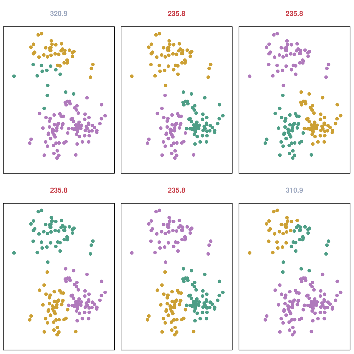
In practice, common to start from many random initializations and choose the output which minimizes the objective function.

Choosing the number of clusters: gap statistic#

Basic idea: after we have discovered all the clusters, the drop in sums of squares will be similar to drops on “null” data.
Requires a model for “null data”: $N(0, I)$? Unif$([-1,1]^p)$?

Choosing the number of clusters: gap statistic#

Rule:

\[ K^* = \text{argmin}_K \left\{K:G(K+1) \geq G(K) + SD_{K+1}\right\} \]

with $SD_{K+1}$ some estimate of the SD.

Extracting features from $K$-means#

Natural features to extract from $K$-means is the cluster assignment

\[ x \mapsto \text{argmin}_{K} \|x - \bar{X}_k\|^2_2 \]

with $\bar{X}_k$ the cluster centers.

Caveats:#

Improvement in prediction does not necessarily imply structure in features.
Real structure in features (i.e. clusters) may not lead to improvement in prediction.

Variants#

Any MDS-type method yields points in Euclidean space
$\implies$ a clean Pipeline…

SpectralClustering = Pipeline([('embed', SpectralEmbedding(n_components=3)),
                               ('clust', KMeans(n_clusters=5))])

Mixture modeling#

A soft clustering algorithm.
Within class model $f_j(X;\theta_j), 1 \leq j \leq K$.
As it is a generative model we have a likelihood we can use for choosing $K$ by BIC / AIC, etc.
Corresponds to hierarchical model with latent labels $Z$:

\[\begin{split} \begin{aligned} Z_i &\sim \text{Multinomial}(\pi) \\ X_i | Z_i=j &\sim f_j(\cdot, \theta_j) \end{aligned} \end{split}\]

Fit by well-known EM algorithm.

EM steps#

E-step: given current values $\tilde{\Theta}=(\tilde{\theta}_1, \dots, \tilde{\theta}_K, \tilde{\pi}_1, \dots, \tilde{\pi}_K)$

\[\begin{split} \begin{aligned} \hat{\gamma}_{ij} &= \hat{\gamma}_{ij}(X_i;\tilde{\Theta}) \\ &= P_{\tilde{\theta}}(Z_i=j|X=X_i) \\ &= \frac{\tilde{\pi}_j f_j(X_i;\tilde{\theta}_j)}{\sum_{l=1}^k \tilde{\pi}_l f_l(X_i; \tilde{\theta}_l)}\\ \end{aligned} \end{split}\]

M-step (when no constraints on $\theta_j$ i.e. not shared across components):

\[\begin{split} \begin{aligned} \hat{\pi}_j &= \frac{1}{n} \sum_{i=1}^n \hat{\gamma}_{ij} \\ \hat{\theta}_j &= \text{argmax}_{\theta_j} \sum_{i=1}^n \hat{\gamma}_{ij} \ell_j(X_i; \theta_j) \end{aligned} \end{split}\]

Choices to be made for mixture#

We must choose a $K$ (BIC / AIC?)
If $f(\cdot, \theta_j) = N(\mu_j, \Sigma_j)$ we still need to choose a model for $\Sigma_j$ between and within classes.
Between classes: typically choice is common or class-specific covariance?
If the same, update for $\Sigma=\Sigma_j$ is a pooled estimate of covariance with weights…

Feature extraction#

Responsibilities $\widehat{\gamma}_j$ can replace $K$-means’ classification rule as features…

Relation with $K$-means#

If we stick with common covariance $\sigma^2 I$ and send $\sigma^2 \to 0$, we see

\[ \hat{\gamma}_{ij}(X;\tilde{\Theta}) \to \delta_{\hat{j}(X_i)} \]

with

\[ \hat{j}(X_i) = \text{argmin}_j \|X_i - \mu_j\|^2_2 \]

Model-based clustering#

Library mclust in R.
Or GaussianMixture.predict()

Using `GaussianMixture` to cluster#

$K$-medoid clustering#

$K$-means / Gaussian mixture models produce centroids that “represent” each cluster as a prototype.
Both rely on Euclidean structure in order to compute centroids: they are (weighted) class averages…
$K$-medoid chooses instead a sample point as the prototype: given cluster $\{X_j:j \in C\}$ and metric $d$ the medoid is

\[ i^*_C = \text{argmin}_{j \in C} \sum_{i \in C} d(X_i, X_j) \]

Assignment step is the same as $K$-means.
Some variants of the assignment / swap step that are not exactly like $K$ means (I believe these variants are used by pam below).
In Euclidean case, said to be more robust because we use norms instead of squared norms.
from sklearn_extra.cluster import KMedoids

Hierarchical clustering#

Most algorithms for hierarchical clustering are bottom up.
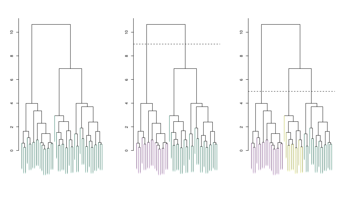
Agglomerative process summarized by a dendrogram.

Clustering is completely determined by initial distance (or dissimilarity) matrix and the choice of dissimilarity between clusters.
The number of clusters is not fixed: each cut of the dendrogram induces a clustering.
At each step, we link the 2 clusters that are closest (least dissimilar) to each other.
Hierarchical clustering algorithms are classified according to the notion of distance between clusters.

Complete linkage: The distance between 2 clusters is the maximum distance between any pair of samples, one in each cluster.
Single linkage: The distance between 2 clusters is the minimum distance between any pair of samples, one in each cluster.
Single linkage suffers from the chaining phenomenon.
Single linkage enjoys a continuity property the others are not known to.
Average linkage: The distance between 2 clusters is the average of all pairwise distances.

Complete linkage#

Average linkage#

Single linkage#

Choices to make#

Because it is so general, there are many choices to make in hierarchical clustering.
Choice of initial dissimilarity matrix is obviously important: e.g. do we measure distance modulo scale?

\[ d_{ij} = \|X_i - X_j\|_2, \qquad \tilde{d}_{ij}=\cos^{-1}\left(\frac{X_i^TX_j}{\|X_i\|_2 \|X_j\|_2} \right) ? \]

Choice of linkage also clearly makes a difference.

Some properties of hierarchical clustering#

Single, complete and average linkage have no inversions: heights when parents are merged are higher than any of their children.
Both single and complete are monotone: monotone transformations of the distances do not change structure of the trees. Not necessarily true for average linkage.
Both single and complete ignore duplicates: duplications of points do not change the structure of the true – many merges happen at height 0. Not necessarily true for average linkage.

Hierarchical clustering with prototypes: minimax linkage#

One of the nice features about $K$-means / $K$-medoids / mixture modeling is that each cluster has a simple representative: $\implies$ useful for downstream tasks…
Bien and Tibshirani consider a different dissimilarity between clustering: minimax linkage
Based on

\[\begin{split} \begin{aligned} d_{\max}(x,C) &= \max_{y \in C} d(x,y) \\ r(C) &= \min_{x \in C} d_{\max}(x,C) \end{aligned} \end{split}\]

with the minimizer in determining $r(C)$ the prototype for $C$.

Dissimilarity between clusters $$ D(G,H) = r(G \cup H) $$
This linkage is monotone, ignores density and has no inversions.

Source: Bien and Tibshirani

Clustering

Contents

Clustering#

Download#

Clustering#

Basic approaches#

\(K\)-means clustering#

Without scaling#

With scaling#

\(K\)-means clustering algorithm#

\(K\)-means output with different initializations#

Choosing the number of clusters: gap statistic#

Choosing the number of clusters: gap statistic#

Extracting features from \(K\)-means#

Caveats:#

Variants#

Mixture modeling#

EM steps#

Choices to be made for mixture#

Feature extraction#

Relation with \(K\)-means#

Model-based clustering#

Using `GaussianMixture` to cluster#

\(K\)-medoid clustering#

Hierarchical clustering#

Complete linkage#

Average linkage#

Single linkage#

Choices to make#

Some properties of hierarchical clustering#

Hierarchical clustering with prototypes: minimax linkage#

Clustering

Contents

Clustering#

Download#

Clustering#

Basic approaches#

\(K\)-means clustering#

Without scaling#

With scaling#

\(K\)-means clustering algorithm#

\(K\)-means output with different initializations#

Choosing the number of clusters: gap statistic#

Choosing the number of clusters: gap statistic#

Extracting features from \(K\)-means#

Caveats:#

Variants#

Mixture modeling#

EM steps#

Choices to be made for mixture#

Feature extraction#

Relation with \(K\)-means#

Model-based clustering#

Using GaussianMixture to cluster#

\(K\)-medoid clustering#

Hierarchical clustering#

Complete linkage#

Average linkage#

Single linkage#

Choices to make#

Some properties of hierarchical clustering#

Hierarchical clustering with prototypes: minimax linkage#

Using `GaussianMixture` to cluster#