Discriminant analysis#
Download#
Classification / Discriminant Analysis#

Setup for *DA#
Given \(K\) classes in \(\mathbb{R}^p\), represented as densities \(f_i(x), 1 \leq i \leq K\) we want to classify \(x \in \mathbb{R}^p\).
In other words, partition \(\mathbb{R}^p\) (or other sample space) into subsets \(\Pi_i, 1 \leq i \leq k\) based on the densities \(f_i(x)\).
We’ll focus on classical methods: LDA and generalizations.
LDA is a misnomer: it is a generative classifier rather than discriminative classifier.
Why is this multivariate analysis?#
Approximations to LDA (e.g. Fisher’s linear discriminant) are connected to CCA and reduced rank regression.
Maximum likelihood rule#
Classify \(x\) to class for which density / likelihood is highest
Bayes rule#
If prior class probabilities \((\pi_1, \dots, \pi_K)\) are available, a more sensible rule is
Optimality of Bayes rule#
Of all discriminant rules \(\delta: \mathbb{R}^p \to {\cal S}_K\), the simplex in \(\mathbb{R}^k\) (i.e. rules which assign points \(x \in \mathbb{R}^p\) a probability on \(\{1,\dots,K\}\)) none has higher probability of correct assignment than the Bayes rule.
A simple discriminant function#
Suppose the sample space is all \(p\)-tuples of integers that sum to \(n\).
Two classes \(f_1 = \text{Multinom}(n, \alpha)\), \(f_2 = \text{Multinom}(n, \beta)\).
ML rule boils down to
The function
is called a discriminant function between classes 1 & 2 (though it is derived from a generative model…)
Discriminant functions#
Set
ML rule can be summarized as
Bayes rule can be summarized as
Example: Gaussian in \(\mathbb{R}\)#
Let \(f_1 = N(\mu_1, \sigma^2_1)\), \(f_2 = N(\mu_2, \sigma^2_2)\).
Discriminant function for Bayes rule:
Note that \(h_{12}\) is quadratic in \(x\), unless \(\sigma_1=\sigma_2\).
LDA (Linear Discriminant Analysis): \(\sigma_1=\sigma_2\)
QDA (Quadratic Discriminant Analysis): \(\sigma_1 \neq \sigma_2\).
Example: Gaussian in \(\mathbb{R}^p\)#
In general, ML rule classifies \(x\) by minimizing Mahalanobis distance (after adjusting for \(\Sigma_i\))
If \(\Sigma_i=\Sigma\) for all \(i\), the ML (LDA) rule classifies by minimizing Mahalanobis distance.
Bayesian rule (with \(\Sigma_i=\Sigma\)) classifies by
so classes with smaller prior probabilities get penalized.
Sample ML and Bayesian rules#
For each class, estimate \((\widehat{\mu}_i, \widehat{\Sigma}_i, \widehat{\pi}_i)\) with \(\widehat{\pi}_i = n_i/n\).
QDA (sample version)#
Classify according to
LDA (sample version)#
First, estimate a pooled covariance matrix
Classify according to $\( x \in \widehat{\Pi}_i \iff i = \text{argmin}_{j} \Delta_{\widehat{\Sigma}_P}(x, \widehat{\mu}_j) - 2 \log \widehat{\pi}_j.\)$
Effective dimension for LDA#
Suppose that \(p > K\), and let $\( L = \mu_1 \oplus \text{span}\{\mu_i - \mu_1, 2 \leq i\leq K\} \)$
It is clear that all of the action happens along affine subspace \(L \subset \mathbb{R}^p\) of dimension at most \((K-1)\).
Suggests we can / should reduce dimension …
Fisher’s linear discriminant#
Given a data matrix \({X}_{n \times p}\) and labels \(L \in \{1,\dots,K\}^n\) consider a linear combination \(Xv\)
The SSE of \(Xv\) can be decomposed as
Fisher’s intuition#
Directions \(v\) with high between variance should be important for classification.
Candidate for a good direction
i.e. maximize between groups variance subject to within group variance of 1.
Characterization of discriminants#
Yields a generalized eigenvalue problem
Can construct up to \(K-1\) different directions (subject \(\widehat{v}_i'\widehat{\Sigma}_W \widehat{v}_j = \delta_{ij}\)).
Define the Fisher discriminant scores
Stack as columns to form a new data matrix \({V}_{n \times (K-1)}\).
First two sample discriminants for iris#
Classification with derived features#
The pooled covariance matrix of the \(V_i\)’s will be \(I\) so LDA is just classifying to the nearest centroid (by Euclidean distance)
Centroids form a (simple) Voronoi diagram on \(\mathbb{R}^{K-1}\)

Source: Wikipedia
Fisher’s linear discriminant & CCA#
Consider the one-hot matrix
We can put the data matrices \({Y}, {X}\) through CCA yielding \(K-1\) pairs \((\widehat{a}_i, \widehat{b}_i), 1 \leq i \leq K-1\) of canonical directions.
It turns out that \(\widehat{b}_i = \widehat{v}_i\) (up to a scalar multiple)…
Eigenproblem for CCA#
Compare to eigenproblem for Fisher’s discriminant#
Dimension reduction#
Suppose some of the \(\mu_i\)’s are collinear $\( \text{dim}(L) < K-1 \)$
Then, some of the Fisher scores will have little information.
We can discard some of the scores and then classify according to the nearest centroid of reduced space.
Really, to classify, we just need good centroids and some covariance for use in Mahalanobis distance.
Glass identification dataset#
Cross-validation to pick n_components?#
sklearnignoresn_componentsinfitandpredict… see documentation
Solution / hack: use LDA as a transform#
Generalizations#
Usual generalizations apply:
create new features
regularize covariance estimates
impose structure on discriminant functions
Nonlinear decision boundaries#
If we transform \(X \in \mathbb{R}^p\) to \(f(X) \in \mathbb{R}^q\), LDA on \(f(X)\) will produce boundaries that are linear in the components of \(f(X)\).
For example, suppose \(p=2\), take \(f(x)=(x_1, x_2, x_1^2, x_2^2, x_1x_2)\).
This will produce discriminant functions $\( f_{ij}(x) = a_{ij,1} x_1 + a_{ij,2} x_2 + a_{ij,3} x_1^2 + a_{ij,4} x_2^2 + a_{ij,5} x_1 x_1 + c_{ij} \)$
Cheap way to get quadratic boundaries, not exactly QDA.
Using quadratic functions for LDA#
library(mda)
data(iris)
data(glass)
glass.quad = mda::fda(Type ~ ., method=polyreg, degree=2, data=glass)
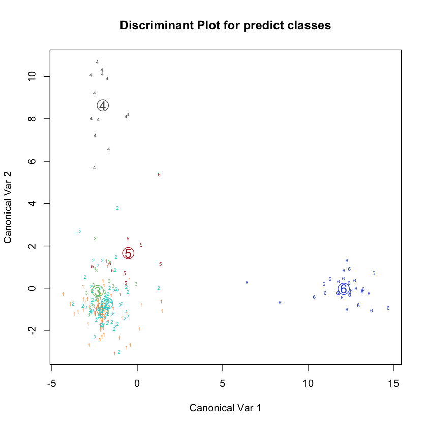
plot(glass.quad)
confusion(glass.quad)
Loading required package: class
Loaded mda 0.5-5
         true
predicted  1  2  3  5  6  7
        1 53 15  3  0  0  0
        2 14 60  2  0  0  0
        3  3  1 12  0  0  0
        5  0  0  0 13  0  0
        6  0  0  0  0  9  0
        7  0  0  0  0  0 29
Using sklearn#
Do quadratic features help?#
More general expansions#
Why limit ourselves to quadratic?
We could take a large basis \(f(x)=(f_1(x), \dots, f_m(x))\) and perform LDA on \(f({X})\) with labels \(L\).
If we take all \(K-1\) fisher scores, the number of coefficients we need to estimate is \((K-1) * m\) – this grows quickly.
We may also have to invert large matrices… regularize?
Does covariance regularization help?#
How about regularization & quadratic features?#
Mixture discriminant analysis#
LDA / Fisher’s method presumes that a single centroid (and common spread) is sufficient to describe a class.
Within class densities are \(N(\mu_j,\Sigma)\)…
A richer model could use a mixture for within class density:
Or use common \(\Sigma_{jl}=\Sigma\)…
Can run EM within each class to fit a mixture. Given the mixture, the Bayes or ML rule is easy…
ESL describes this as a compromise between LDA and nearest-neighbor classifier.
3 components per class#
#| echo: true
glass.lda = mda::fda(Type ~ ., data=glass)
glass.mda = mda::mda(Type ~ ., data=glass, subclasses=3)
glass.mda
accuracy = function(C_) { sum(diag(C_))/sum(C_) }
accuracy(confusion(glass.mda))
accuracy(confusion(glass.lda))
Call:
mda::mda(formula = Type ~ ., data = glass, subclasses = 3)

Dimension: 9

Percent Between-Group Variance Explained:
    v1     v2     v3     v4     v5     v6     v7     v8     v9
 72.43  84.70  92.40  95.99  97.80  98.88  99.43  99.74 100.00

Degrees of Freedom (per dimension): 10

Training Misclassification Error: 0.25234 ( N = 214 )

Deviance: 338.763
Combining dimension reduction & mixtures#
First, project to lower dimension and then fit mixture model
#| echo: true
glass.mda4 = mda(Type ~ ., data=glass, subclasses=3, dimension=4)
glass.mda4
accuracy(confusion(glass.mda4))
Call:
mda(formula = Type ~ ., data = glass, subclasses = 3, dimension = 4)

Dimension: 4

Percent Between-Group Variance Explained:
   v1    v2    v3    v4
78.76 88.59 94.82 97.59

Degrees of Freedom (per dimension): 10

Training Misclassification Error: 0.25701 ( N = 214 )

Deviance: 335.744
Does dimension reduction have any effect for MDA?#
#| echo: true
set.seed(1)
samp = sample(1:214, 100, replace=FALSE)
glass.test = glass[samp,]
glass.train = glass[-samp,]
glass.mda = mda(Type ~ ., data=glass.train, subclasses=3)
glass.mda4 = mda(Type ~ ., data=glass.train, subclasses=3, dimension=4)
accuracy(confusion(glass.mda, glass.test))
accuracy(confusion(glass.mda4, glass.test))
Naive Bayes#
As in CCA, we must implicitly invert \(\hat{\Sigma}_W\) to compute Fisher’s score (or to fit LDA).
We can simplify the model by assuming that \(\Sigma_j\) is diagonal in QDA – this leads to Naive Bayes
For continuous features, default is
Naive Bayes as covariance regularization#
Assuming a diagonal covariance is form of regularization on the covariance…
ESL also defines Diagonal LDA – use common diagonal covariance.
Other regularized covariance estimates#
or
Choice of tuning parameters#
Since we are classifying, we can use cross-validation…
Shrunken centroids#
One can also regularize the centroid estimates.
Neareast Shrunken Centroids combines diagonal LDA with regularization.
For each feature \(l\), soft-threshold \(\bar{X}_{j,l} - \bar{X}_l\) (or more precisely the \(Z\)-scores).
Forces many features to share common centroid value \(\hat{\mu}_{j,l}\) – means they effectively do not contribute to classification rule
Nearest shrunken centroids#

(Source: ESL)