Hotelling T2#
Download#
Two-sample tests#

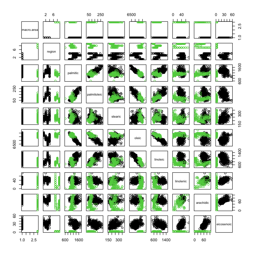
Olive oil data#
#| echo: true
library(pdfCluster)
data(oliveoil)
# let's make it a two-sample dataset (of 3 regions)
X = oliveoil[oliveoil$macro.area %in% c('South', 'Centre.North'),]
pairs(X, col=X$macro.area)
pdfCluster 1.0-4
North vs. south#
#| echo: true
South = X[X$macro.area=='South',3:10]
North = X[X$macro.area=='Centre.North',3:10]
X_1 = South
X_2 = North
Two-sample tests: model#
Consider \(X_1 \in \mathbb{R}^{n_1 \times p}\) an \(N(\mu_1, \Sigma_1)\) data matrix and \(X_2 \in \mathbb{R}^{n_2 \times p}\) and \(N(\mu_2, \Sigma_2)\) data matrix.
Assuming \(\Sigma_1=\Sigma_2\) we consider testing \(H_0: \mu_1=\mu_2\).
Hotelling’s \(T^2\) test#
Obvious (?) candidate
with
Under \(H_0: T^2 \sim \frac{mp}{m-p+1} F_{p,m-p+1}\)
Computing the test statistic#
#| echo: true
n_1 = nrow(X_1)
n_2 = nrow(X_2)
p = ncol(X_1)
S_p = (((n_1 - 1) * cov(X_1) + (n_2 - 1) * cov(X_2))
       / (n_1 + n_2 - 2))
diff = apply(X_1, 2, mean) - apply(X_2, 2, mean)
T2 = n_1 * n_2 / (n_1 + n_2) * t(diff) %*% solve(S_p) %*% diff
m = n_1 + n_2 - 2
F = (m - p + 1) / (p * m) * T2
pvalue = 1 - pf(F, p, m - p + 1)
data.frame(F=F, T2=T2, num=p, denom=m-p+1, pvalue)
| F | T2 | num | denom | pvalue |
|---|---|---|---|---|
| <dbl> | <dbl> | <int> | <dbl> | <dbl> |
| 405.3333 | 3291.481 | 8 | 465 | 0 |
Using a package#
#| echo: true
library(Hotelling)
T = hotelling.test(X_1, X_2)
print(T)
T$stats
Loading required package: corpcor
Test stat:  3291.5
Numerator df:  8
Denominator df:  465
P-value:  0
- $statistic
- 3291.48078049422
- $m
- 0.123146186440678
- $df
-
- 8
- 465
- $nx
- 323
- $ny
- 151
- $p
- 8
A harder test#
#| echo: true
set.seed(0)
split_ = sample(1:nrow(South), 150, replace=FALSE)
X_1H = South[split_,]
X_2H = South[-split_,]
T = hotelling.test(X_1H, X_2H)
print(T)
Test stat:  3.2509
Numerator df:  8
Denominator df:  314
P-value:  0.9216
Distribution of test statistic#
Easy to see under \(H_0\)
with
Largest \(t\) statistic interpretation#
Let
Then,
Quick check
Alternatively,
Asymptotic behavior#
As \(n_1, n_2 \to \infty\) and \(S_p \to \Sigma\) (recall we assume \(\textrm{Var}(X_1)=\textrm{Var}(X_2))\). Plugging in…
under \(H_0: E(X_1)=E(X_2)\) (and equal variances).
Equal variances?#
pairs(X, col=X$macro.area)
Calibration using permutation#
#| echo: true
T = hotelling.test(X_1, X_2, perm=TRUE, progBar=FALSE)
T
Test stat:  405.33
Numerator df:  8
Denominator df:  465
Permutation P-value:  0
Number of permutations : 10000
Harder version#
#| echo: true
T = hotelling.test(X_1H, X_2H, perm=TRUE, progBar=FALSE)
T
Test stat:  0.3975
Numerator df:  8
Denominator df:  314
Permutation P-value:  0.9223
Number of permutations : 10000
Alternative tests#
Instead of maximizing over \(\{a: a^T\Sigma a \leq 1\}\) might consider analog of Bonferroni (over coordinate directions \(e_j\))
Or,
with \(Z \sim N(0, I_{p \times p})\).
Calibrating tests: Roy’s union-intersection principle (5.2.2 of MKB)#
For simplicity let’s take \(n_1, n_2 \gg 1\) and \(\Sigma=I\)
Null hypothesis is an intersection
with
Suppose that for each \(a \in A\) we have a test statistic to test \(H_{0,a}\) (under \(n_1, n_2 \gg 1\))
Consider rejection regions that are unions
Most common to pick \(z_{\alpha}\) chosen so that under \(H_0\)
Back to Hotelling’s \(T^2\)#
Returning to finite samples, Hotelling’s \(T^2\) test uses \(t^2(a; X_1, X_2)\) with pooled estimate of covariance for each direction \(a\). Cutoff chosen from relation to \(F\) distribution…
For two alternative tests presented, calibration must be done by bounding (i.e. Bonferroni bound), simulation (including permutation) or more careful analysis.
Another look at Hotelling \(T^2\)#
Let’s stack the data to form
Rewriting the statistic#
Let $\( M_1 = \frac{1}{n_1} \begin{pmatrix} 1_{n_1} \\ 0_{n_2} \end{pmatrix}, \qquad M_2 = \frac{1}{n_2} \begin{pmatrix} 0_{n_1} \\ 1_{n_2} \end{pmatrix}. \)$
Difference of means is
\(T^2\) as a trace#
Differencing projection#
Numerical check#
#| echo: true
X = as.matrix(rbind(X_1, X_2))
n_1 = nrow(X_1)
n_2 = nrow(X_2)
M_1 = c(rep(1, n_1), rep(0, n_2)) / n_1
M_2 = c(rep(0, n_1), rep(1, n_2)) / n_2
P_delta = (M_1 - M_2) %*% t(M_1 - M_2) * n_1 * n_2 / (n_1 + n_2)
S_p = ((n_1 - 1) * cov(X_1) + (n_2 - 1) * cov(X_2)) / (n_1 + n_2 - 2)
T2_alt = sum(diag(X %*% solve(S_p) %*% t(X) %*% P_delta))
c(T2, T2_alt)
- 3291.48078049422
- 3291.48078049758
Form of the test statistic#
Take any symmetric \(G\) $\( G = \begin{pmatrix} G_{11} & G_{12} \\ G_{21} & G_{22} \end{pmatrix} \)$
The statistic takes the form $\( \begin{aligned} \text{Tr}(GP^{\Delta}) &= \frac{1}{n_1^2} \sum_{i,j=1}^{n_1} G_{11}[i,j] \\ & \qquad - \frac{2}{n_1n_2} \sum_{i=1}^{n_1} \sum_{j=1}^{n_2} G_{12}[i,j] \\ & \qquad + \frac{1}{n_2^2} \sum_{i,j=1}^{n_2} G_{22}[i,j] \\ \end{aligned} \)$
Can be interpreted as (average) within-group similarity minus (average) between-group similarity…
May want to remove diagonal entries (more shortly)
Imagining \(n_1, n_2 \to \infty\) this becomes approximately
where \(G_{n \times n}\) is a Gram matrix (also a similarity) matrix.
With \(p\) large-ish \(\Sigma^{-1}\) might be hard to estimate might just substitute
or even
Different featurization#
Suppose we featurize \(X\) differently, i.e. instead of rows \(X[i,]\) we consider \(h:\mathbb{R}^p \rightarrow\mathbb{R}^k\) a new data matrix
with
Can just as easily “compute” Hotelling \(T^2\) with \(h(X)\) instead of \(X\)
with
with \(S_p^h\) a pooled estimate of covariance from \(h(X)\). Or, might use diagonals only…
Calibration by permutaion#
Under \(H_0: F_1=F_2\) a simple permutation procedure can be used.
First, let’s assume that for some fixed \(h\) (recall that \(X\) is the full data matrix).
Compute our observed test-statistic
Permutation distribution#
For \(B\) independently drawn random permutation \(\sigma\) (viewed as a 0-1 matrix), define
Report \(p\)-value
Some parameters in the Gram matrix \(G\) might depend on \(X\) – under some conditions plugin principle might work, else could recompute \(G\) for each \(\sigma\).
Example#
Let’s add quadratic in
oleicas well if we suspect 2nd moment ofoleicis also different…Moral: the idea from regression of adding extra features can also be used for testing…
#| echo: true
Z_1H = cbind(X_1H, qoleic=X_1H[,'oleic']^2)
Z_2H = cbind(X_2H, qoleic=X_2H[,'oleic']^2)
T = hotelling.test(Z_1H, Z_2H, perm=TRUE, progBar=FALSE)
print(T)
Test stat:  0.3571
Numerator df:  9
Denominator df:  313
Permutation P-value:  0.9526
Number of permutations : 10000