Factor analysis#
Download#
Factor analysis#
Our PPCA model
More generally, we could assume
and \(\Psi\) a diagonal matrix. (Book uses \(\Lambda\) for my \(\Gamma\)).
Probabilistic PCA vs Factor Analysis#
Suppose \(A=\text{diag}(a_1, \dots, a_p)\) then $\( AX \sim N\left(A\mu, A^2 \Psi + A \Gamma \Gamma^TA^T\right) \)$
\(\implies\) a factor model remains a factor model
\(\implies\) not true for PPCA!
If \(R\) is an orthogonal rotation then
\(\implies\) PPCA model is preserved but factor model is not…
Likelihood of factor analysis model#
In the normal model, there is a well-defined likelihood (with \(R_c\) we’ve profiled out \(\mu\)..)
(Negative-log)-likelihood not really amenable to simple algorithms to minimize over \((\Psi,\Gamma)\).
Still, having a log-likelihood opens up AIC / BIC / CV for choosing rank \(k\).
Generative model#
Similar to Probabilistic PCA:
Estimation of factor analysis model#
In the population setting, note that if \(\Psi\) is known
Hence, we might take \(\Gamma = V[,1:k] \Lambda[1:k]^{1/2}\), based on leading rank \(k\) eigendecomposition of \(\Sigma-\Psi\).
Principal factor analysis for rank \(k\)#
Start with initial estimate \(\widehat{\Psi}^{(1)}\) and covariance (or correlation) matrix \(\widehat{\Sigma}\).
For \(i=1,\dots\), run rank \(k\) eigendecomposition on \(\widehat{\Sigma}-\widehat{\Psi}^{(i)}\) yielding
Set
Repeat steps 2. & 3.
Factor analysis for flow data (MLE)#
flow = read.table('http://www.stanford.edu/class/stats305c/data/sachs.data.txt', sep=' ', header=FALSE)
FA_flow = factanal(flow, 2, scores='regression')
names(FA_flow)
FA_flow
- 'converged'
- 'loadings'
- 'uniquenesses'
- 'correlation'
- 'criteria'
- 'factors'
- 'dof'
- 'method'
- 'rotmat'
- 'scores'
- 'STATISTIC'
- 'PVAL'
- 'n.obs'
- 'call'
Call:
factanal(x = flow, factors = 2, scores = "regression")

Uniquenesses:
   V1    V2    V3    V4    V5    V6    V7    V8    V9   V10   V11
0.014 0.005 0.816 0.841 0.998 0.979 0.786 0.955 0.038 0.046 0.315

Loadings:
    Factor1 Factor2
V1   0.121   0.986
V2   0.148   0.987
V3   0.371   0.215
V4   0.352   0.189
V5
V6   0.145
V7   0.389   0.249
V8  -0.164  -0.136
V9   0.978
V10  0.971   0.102
V11  0.822

               Factor1 Factor2
SS loadings      3.072   2.133
Proportion Var   0.279   0.194
Cumulative Var   0.279   0.473

Test of the hypothesis that 2 factors are sufficient.
The chi square statistic is 22471.07 on 34 degrees of freedom.
The p-value is 0
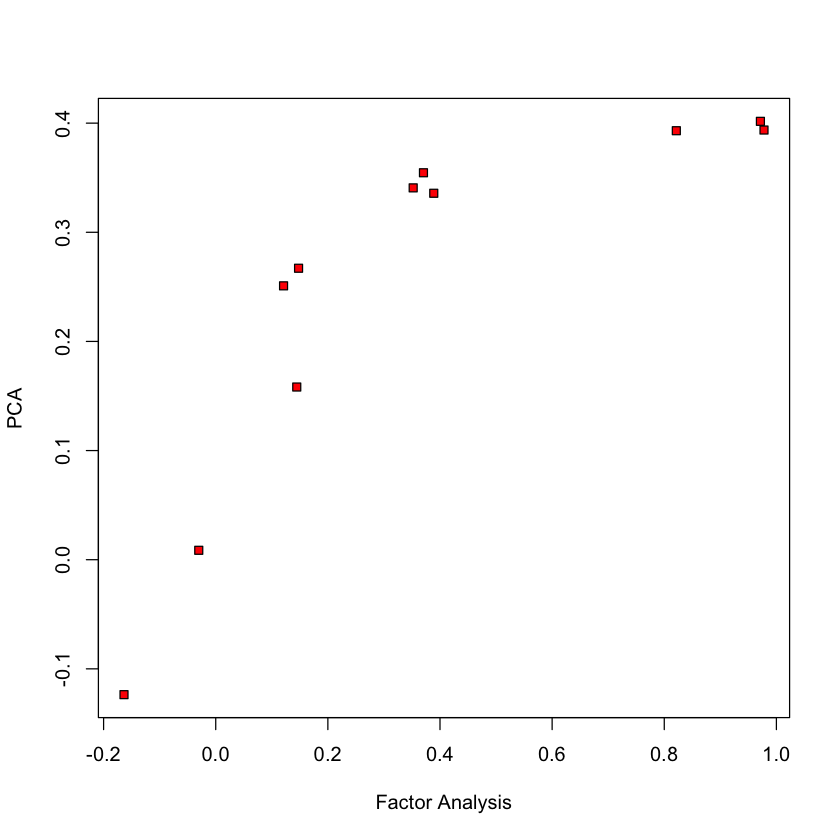
Compare to PCA (1st loading)#
pca_flow = prcomp(flow, center=TRUE, scale.=TRUE)
plot(FA_flow$loadings[,1], pca_flow$rotation[,1], ylab='PCA', xlab='Factor Analysis', pch=22, bg='red')
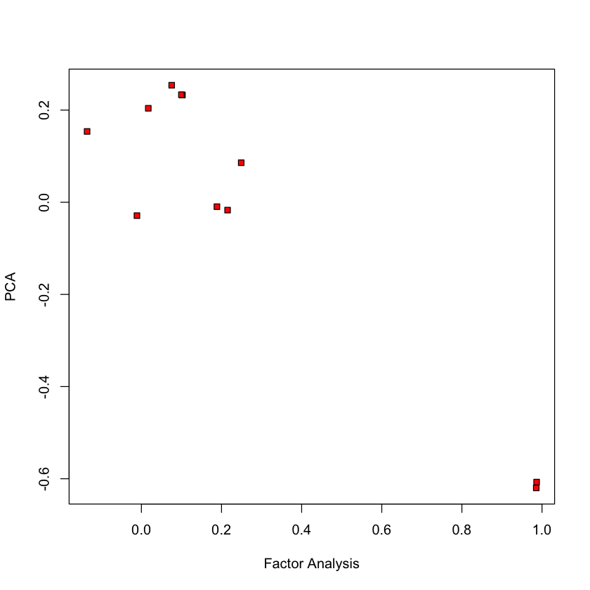
Compare to PCA (2nd loading)#
plot(FA_flow$loadings[,2], pca_flow$rotation[,2], ylab='PCA', xlab='Factor Analysis', pch=22, bg='red')
Latent scores#
Scores \(Z\) are such that
suggesting that, given an estimate \((\Gamma, \Psi)\) we can recover \(Z\) from \(X\) by regression (Bartlett’s scores)
Alternatively (Thomson’s scores)
Thomson has lower MSE, Bartlett’s is unbiased…
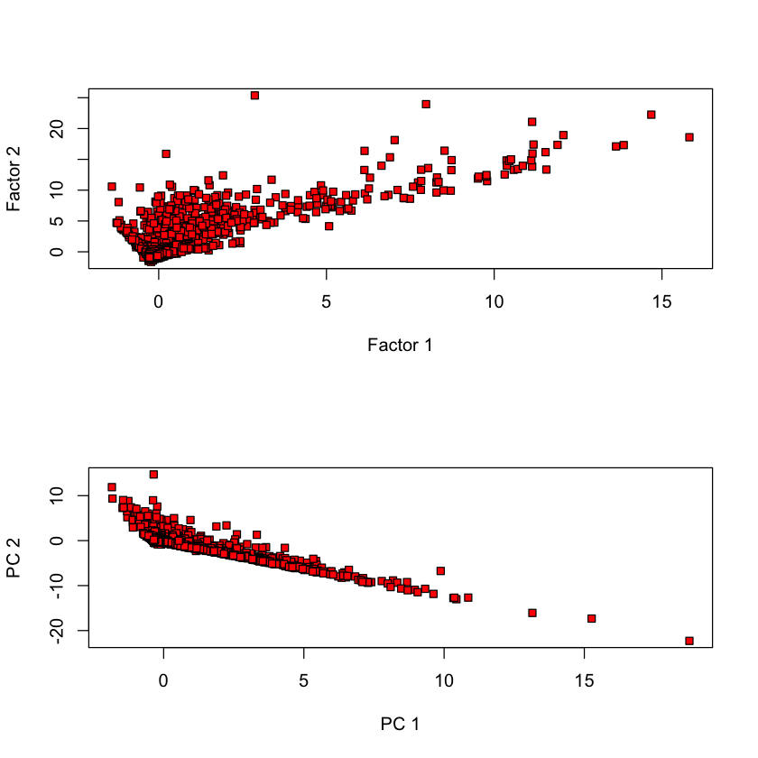
Comparing scores#
par(mfrow=c(2, 1))
plot(FA_flow$scores[,1], pca_flow$x[,1], pch=22, bg='red', xlab='Factor 1', ylab='Factor 2')
plot(FA_flow$scores[,2], pca_flow$x[,2], pch=22, bg='red', xlab='PC 1', ylab='PC 2')
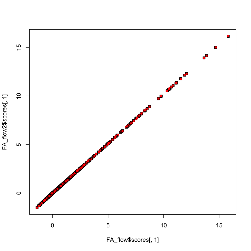
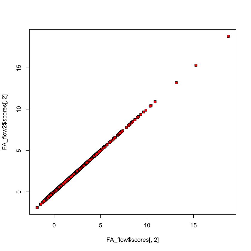
Comparing Thomson vs. Bartlett scores#
FA_flow2 = factanal(flow, 2, scores='Bartlett')
plot(FA_flow$scores[,1], FA_flow2$scores[,1], bg='red', pch=22)
Comparing Thomson vs. Bartlett scores#
plot(FA_flow$scores[,2], FA_flow2$scores[,2], bg='red', pch=22)
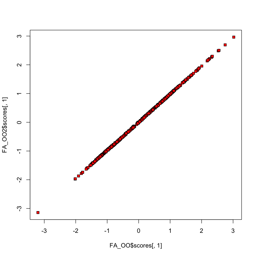
Olive oil data#
#| echo: true
library(pdfCluster)
data(oliveoil)
OO = oliveoil[,3:10]
FA_OO = factanal(OO, 2, scores='Bartlett')
FA_OO2 = factanal(OO, 2, scores='regression')
pdfCluster 1.0-4
plot(FA_OO$scores[,1], FA_OO2$scores[,1], bg='red', pch=22)
How many factors can we fit?#
Remaining degrees of freedom after we fit for \(k\) factors is
MLE can still be challenging for
factanal
#| echo: true
k = 3; p = 11
print(0.5 * ((p - k)^2 - (p + k)))
tryCatch({
  factanal_output <- factanal(flow, k)
}, error = function(e) {
   paste("Factanal failed with k =", k, ". Error:", e$message)
})
[1] 25
Latent variables and EM#
Likelihood is somewhat hard to maximize having observed only \(X\).
BUT, if we observed \(Z\), estimation is easy…
Estimation of \(\Gamma\) would be a multivariate regression of \(X\) onto \(Z\).
Estimation of \(\Psi\) would be easy: take diagonal part of usual MLE of \(\widehat{\Sigma}\) in the above regression.
Suggests EM algorithm is a nice fit for factor analysis…
EM for factor analysis#
Complete (negative) log-likelihood#
Note that \(Z|X \sim N\left(V'(VV' + \Psi)^{-1} X, I - V'(VV' + \Psi)^{-1}V\right)\)
Expected value given \(X\) at \((V_{\text{cur}}, \sigma^2_{\text{cur}}) = (V_c, \sigma^2_c)\) (ignoring irrelevant terms)#
Estimation of new \((V_{\text{new}}, \Psi_{\text{new}})\): multi response regression with covariance \(I_{n \times n} \otimes (\sigma^2 I_{p \times p})\)…
A convex version of factor analysis?#
In the factor analysis model \(\Sigma^{-1}\) also has a particular structure.
For arguments sake, let’s assume \(\Psi=I\) and \(\Gamma^T\Gamma=\kappa I\). Then,
Or, \(\Sigma^{-1}\) is diagonal minus a low-rank (for general case, use Sherman-Morrison-Woodbury.
Let \(\Theta = \Sigma^{-1} = \Phi - \Gamma \Gamma^T = \Phi - \Omega\):
subject to \(\Phi\) being diagonal and \(\Omega\) is rank \(k\) (implicitly \(\Phi - \Omega > 0\))
Convex relaxation#
The rank constraint is not convex but the usual surrogate for rank is nuclear norm
This is convex once we recall that be a valid inverse covariance we must have \(\Phi-\Omega \geq 0\)
Introducing this (convex) constraint yields a convex version of factor analysis
subject to \(\Phi\) being diagonal.
Similar model considered in Chandrasekaran et al. – relaxed diagonal \(\Phi\) to sparse \(\Phi\). Combination of factor analysis and graphical LASSO.